CS50-AI

This blog is used to note down all the knowledge I’ve learned in this lesson.

Here is some links to this lesson.

Home Page and Gradebook

About submitting projects:

check50 , submit50 , my submit , Pass_submit

Here is my solution to labs and the course resources including slides and code ex.

Lecture 0 Search

uninformed search

DFS && BFS

informed search

greedy best-first search

search algorithm that expands the node that is closest to the goal, as estimated by a heuristic function $h(n)$

Heuristic function? Manhattan distance.

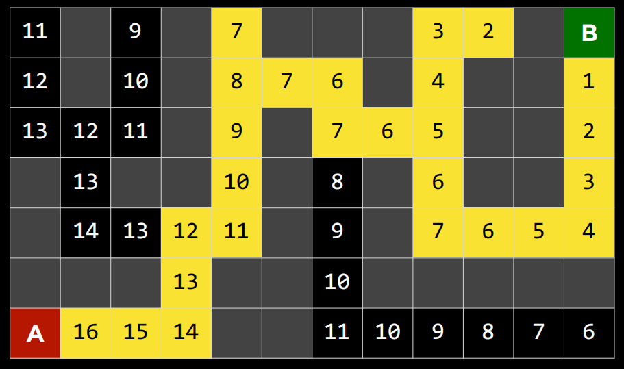
Choose the best way that minimize the heuristic function every time. It makes decision locally.

But this greedy algorithm won’t always find the best way.(The shortest)

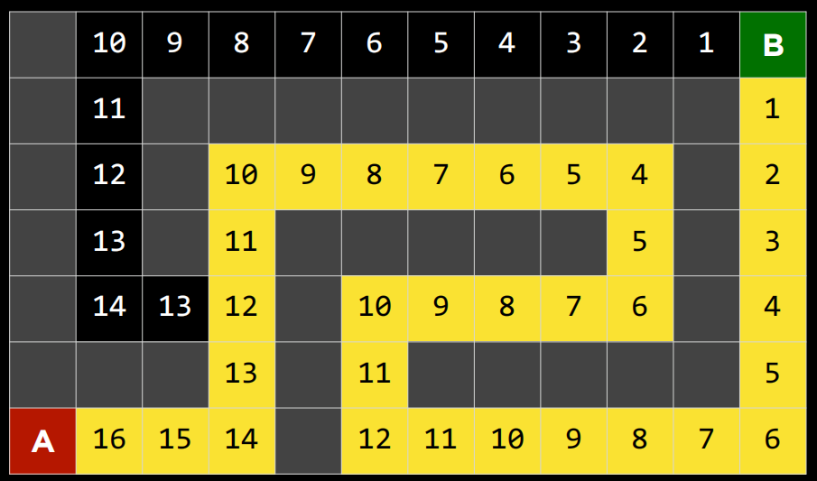
$A^*$ search

search algorithm that expands node with lowest value of $g(n)+ h(n)$

$g(n)$ = cost to reach node

$h(n)$ = estimated cost to goal

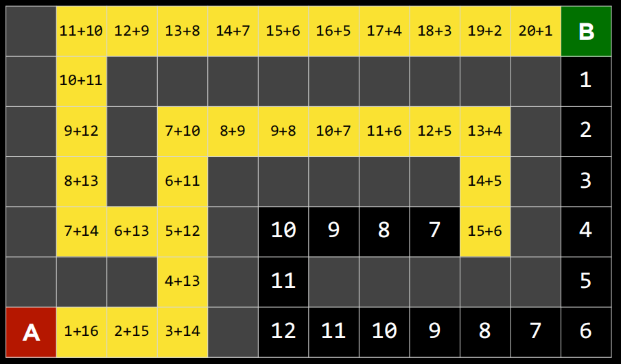
A* search optimal if

• $h(n)$ is admissible (never overestimates the true cost), and

• $h(n)$ is consistent (for every node n and successor n’ with step cost c, h(n) ≤ h(n’) + c)

Adversarial Search

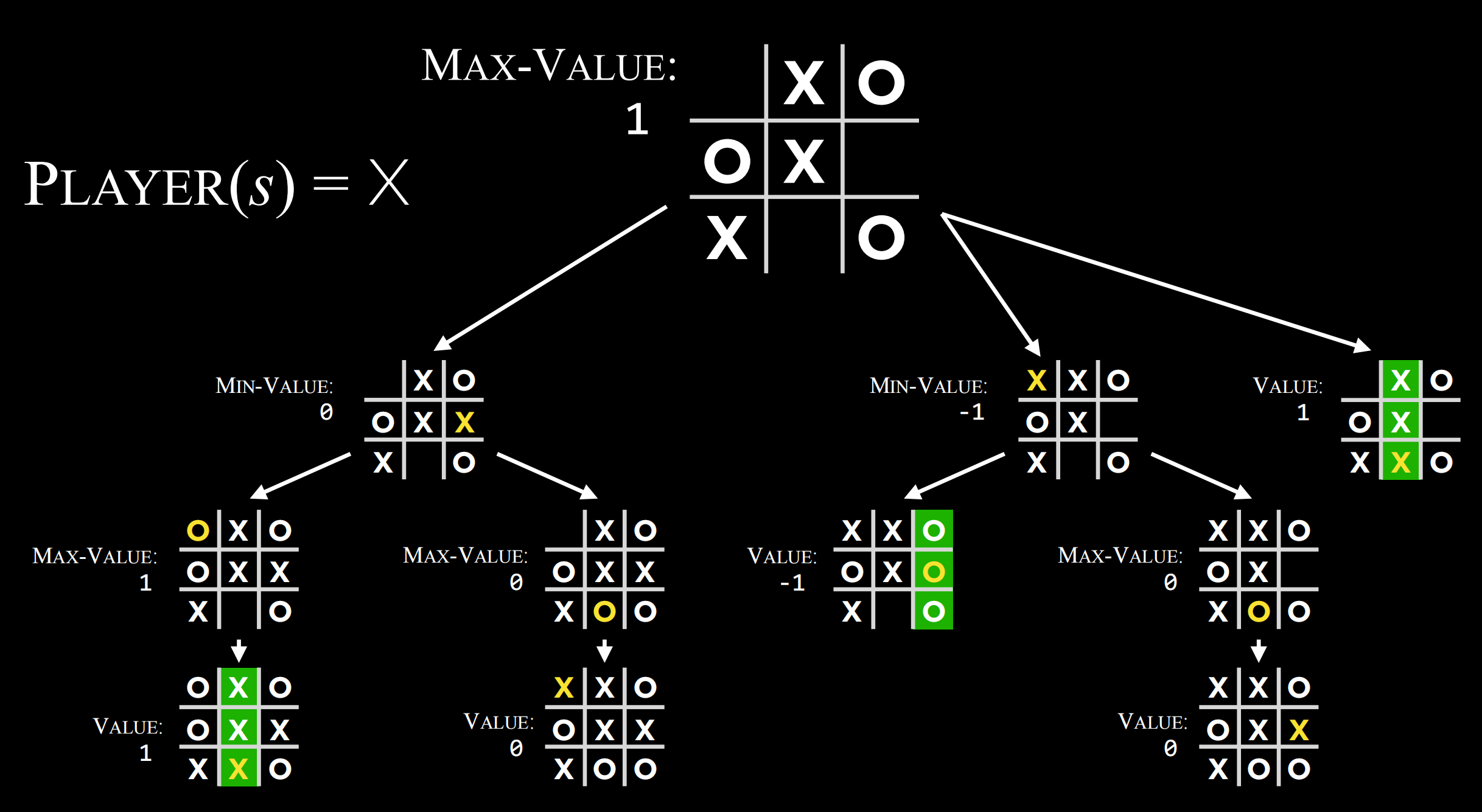
eg.Tic-Tac-Toe

Minimax

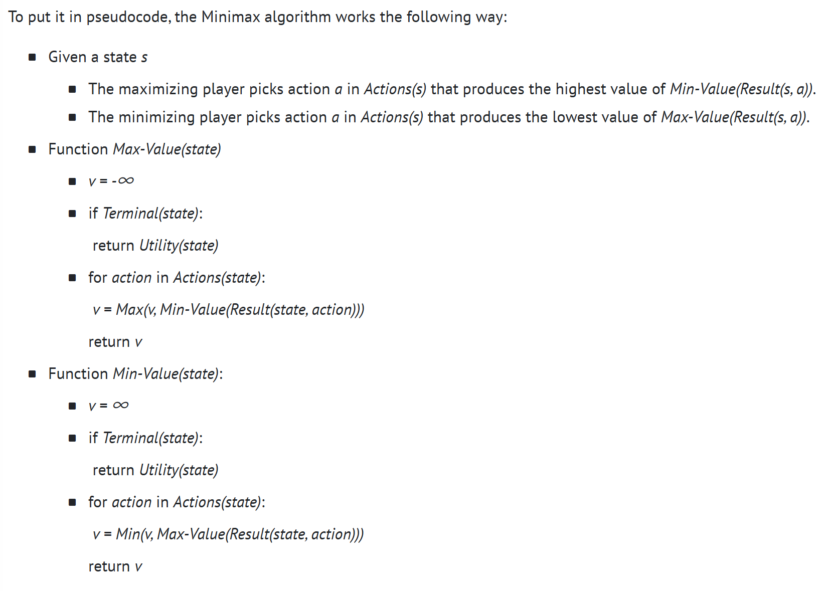
Minimax represents winning conditions as (-1) for one side and (+1) for the other side. Further actions will be driven by these conditions, with the minimizing side trying to get the lowest score, and the maximizer trying to get the highest score.

Alpha-Beta Pruning

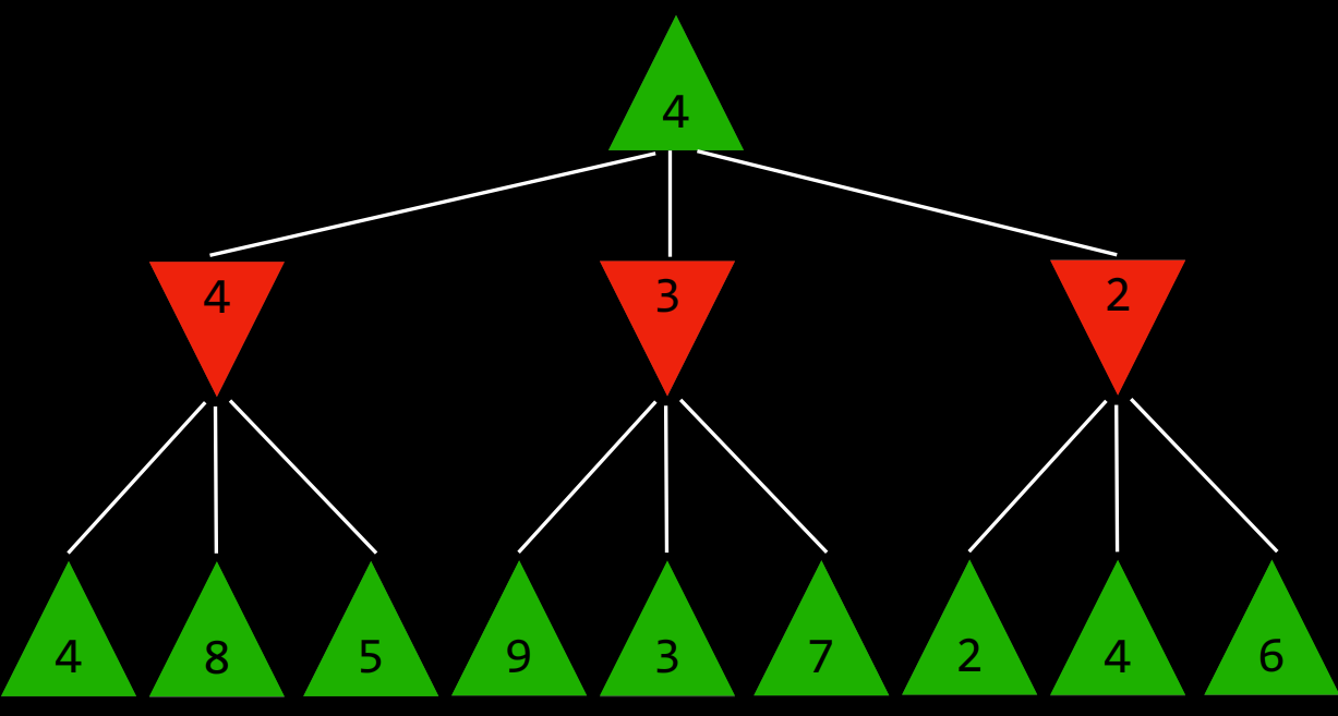
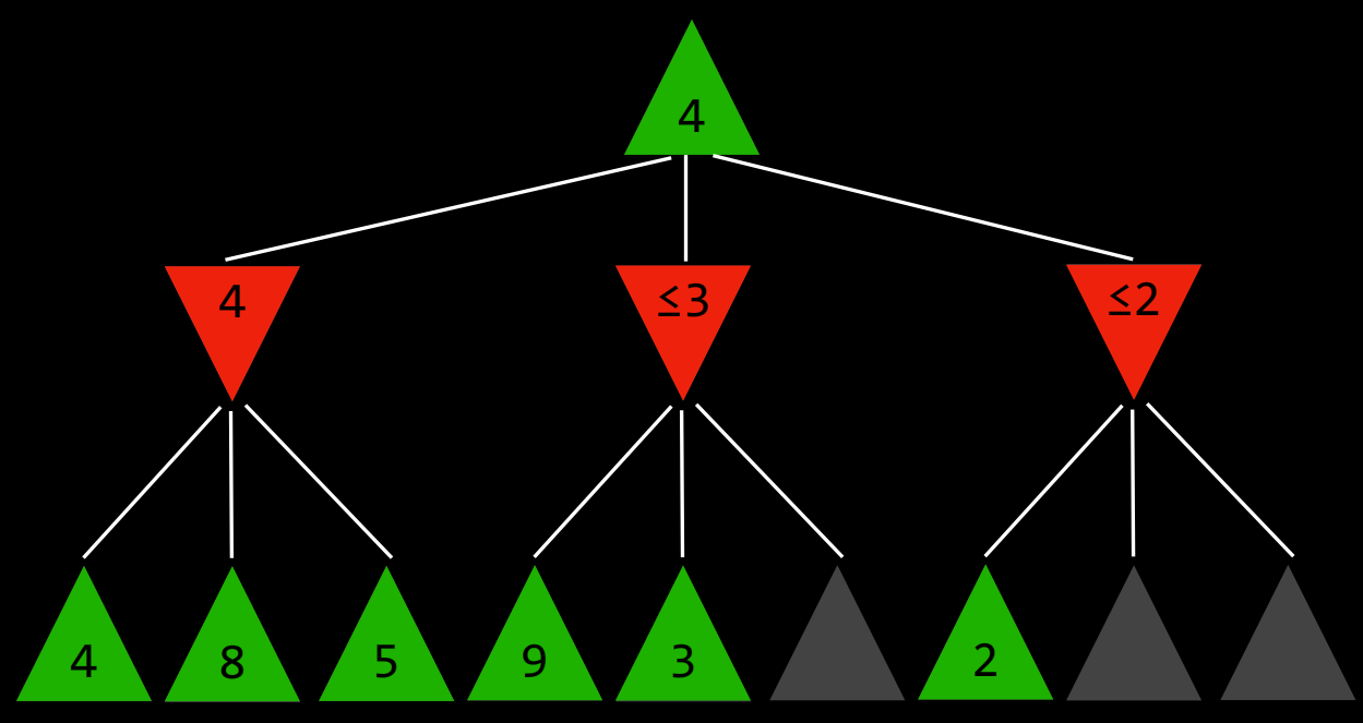
Alpha and Beta are two values that you need to update, which means the best thing you can do so far and the worst thing you can do so far.

Depth-Limited Minimax

need an evaluation function : function that estimates the expected utility of the game from a given state

Lecture 1 Knowledge

Propositional Logic

We’ve learned most of them in Mathematical Logic.

Inference

Model checking

To determine if KB ⊨ α:

• Enumerate all possible models.

• If in every model where KB is true, α is true, then KB entails α.

• Otherwise, KB does not entail α

Knowledge Engineering

Inference Rules

Conjunctive Normal Form

A Clause is a disjunction of literals (a propositional symbol or a negation of a propositional symbol, such as P, ¬P). A disjunction consists of propositions that are connected with an Or logical connective (P ∨ Q ∨ R). A conjunction, on the other hand, consists of propositions that are connected with an And logical connective (P ∧ Q ∧ R). Clauses allow us to convert any logical statement into a Conjunctive Normal Form (CNF), which is a conjunction of clauses, for example: (A ∨ B ∨ C) ∧ (D ∨ ¬E) ∧ (F ∨ G).

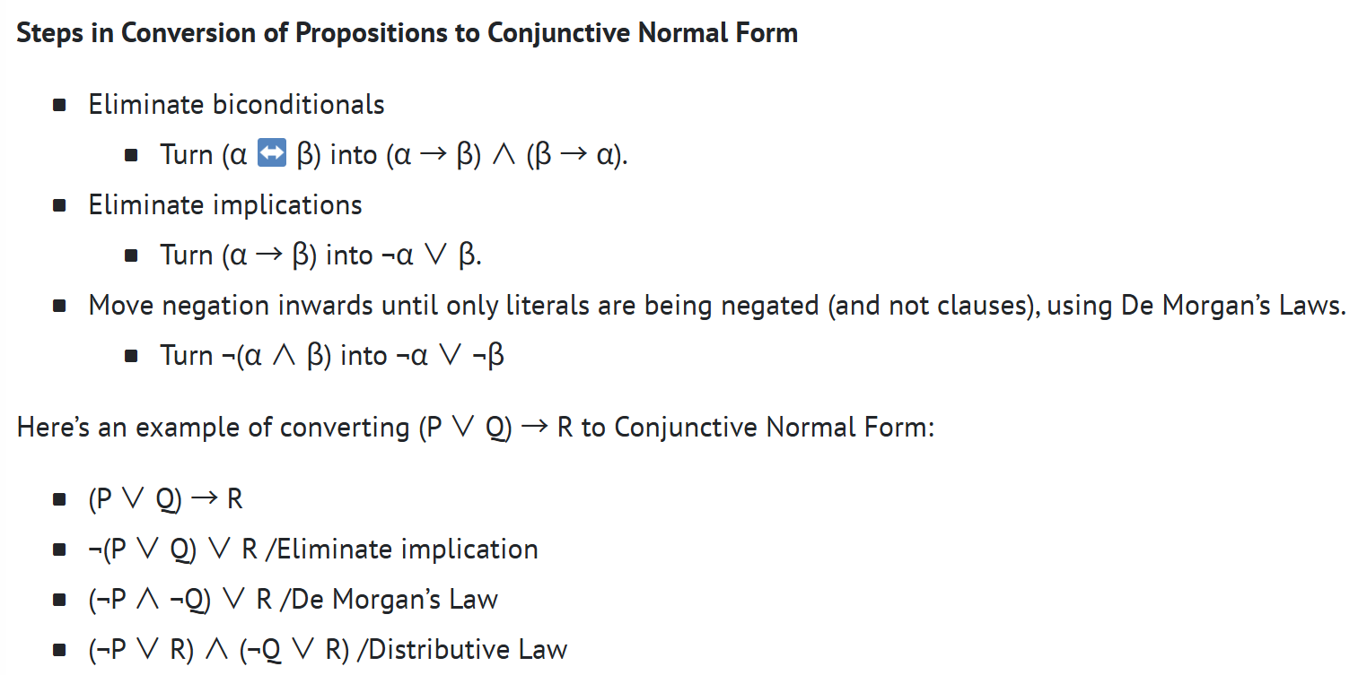
Resolving a literal and its negation, i.e. ¬P and P, gives the empty clause (). The empty clause is always false, and this makes sense because it is impossible that both P and ¬P are true. This fact is used by the resolution algorithm.

• To determine if KB ⊨ α:
  • Check: is (KB ∧ ¬α) a contradiction?
    • If so, then KB ⊨ α.
    • Otherwise, no entailment.

Proof by contradiction is a tool used often in computer science. If our knowledge base is true, and it contradicts ¬α, it means that ¬α is false, and, therefore, α must be true. More technically, the algorithm would perform the following actions:

• To determine if KB ⊨ α:
  • Convert (KB ∧ ¬α) to Conjunctive Normal Form.
  • Keep checking to see if we can use resolution to produce a new clause.
  • If we ever produce the empty clause (equivalent to False), congratulations! We have arrived at a contradiction, thus proving that KB ⊨ α.
  • However, if contradiction is not achieved and no more clauses can be inferred, there is no entailment.

First-Order Logic

Lecture 2 Uncertainty

Conditional probability

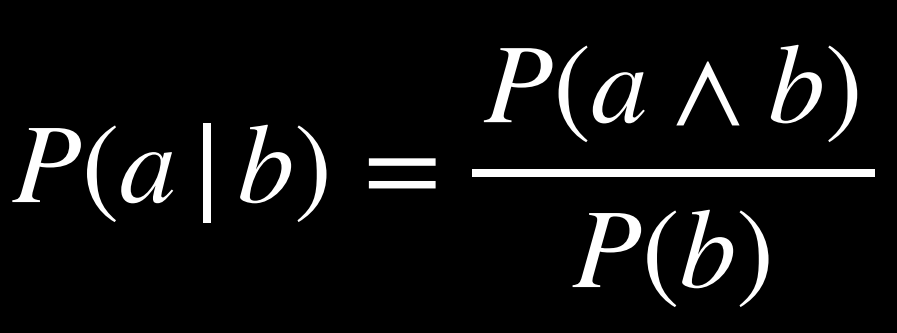
P(a | b), meaning “the probability of event a occurring given that we know event b to have occurred,”

Random Variables

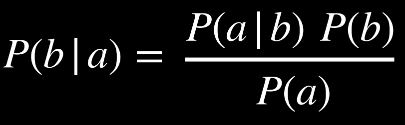
Bayes’ Rule

Conditioning

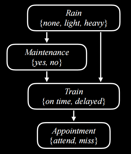
Bayesian Networks

Inferences

Inference by Enumeration

Approximate Inference

Sampling

Likelihood Weighting

• Sample the non-evidence variables using conditional probabilities in the Bayesian network.
• Weight each sample by its likelihood: the probability of all the evidence occurring.

Markov Models

The probability changed due to time changes

The Markov Assumption

the assumption that the current state depends on only a finite fixed number of previous states

Markov chain

a sequence of random variables where the distribution of each variable follows the Markov assumption

To start constructing a Markov chain, we need a transition model that will specify the the probability distributions of the next event based on the possible values of the current event.

Hidden Markov Models

a Markov model for a system with hidden states that generate some observed event

Our AI wants to infer the weather (the hidden state), but it only has access to an indoor camera that records how many people brought umbrellas with them. Here is our sensor model (also called emission model) that represents these probabilities:

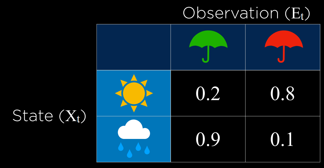
sensor Markov assumption

the assumption that the evidence variable depends only the corresponding state

Lecture 3 Optimization

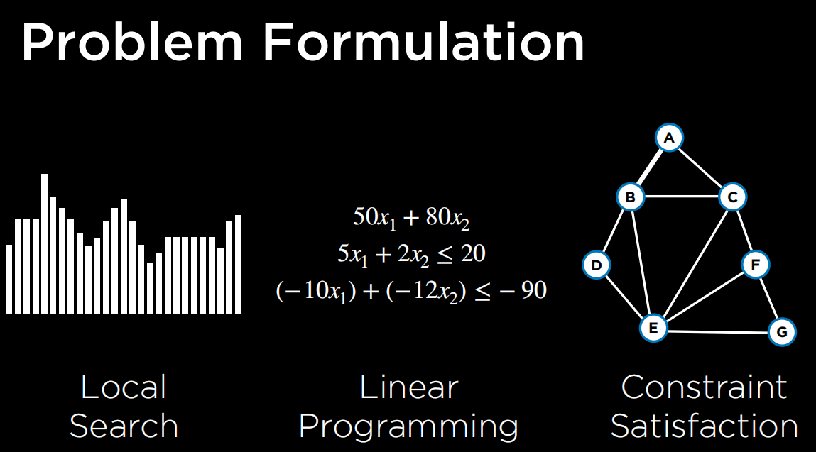
Optimization

choosing the best option from a set of options

local search

search algorithms that maintain a single node and searches by moving to a neighboring node

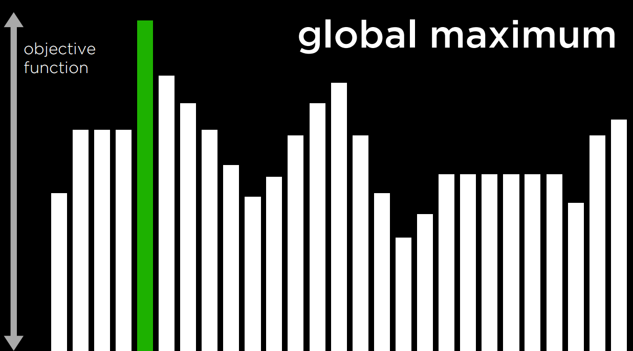
Construct a state-space landscape. We’re going to find the global maximum or global minimum.

Hill Climbing

function Hill-Climb(problem):

• current = initial state of problem
• repeat:
  • neighbor = best valued neighbor of current
  • if neighbor not better than current :
    • return current
  • current = neighbor

Local and Global Minima and Maxima

shoulders, where multiple states of equal value are adjacent and the neighbors of the plateau can be both better and worse

Hill Climbing Variants

• Steepest-ascent: choose the highest-valued neighbor. This is the standard variation that we discussed above.
• Stochastic: choose randomly from higher-valued neighbors. Doing this, we choose to go to any direction that improves over our value. This makes sense if, for example, the highest-valued neighbor leads to a local maximum while another neighbor leads to a global maximum.
• First-choice: choose the first higher-valued neighbor.
• Random-restart: conduct hill climbing multiple times. Each time, start from a random state. Compare the maxima from every trial, and choose the highest amongst those.
• Local Beam Search: chooses the k highest-valued neighbors. This is unlike most local search algorithms in that it uses multiple nodes for the search, and not just one.

Simulated Annealing

function Simulated-Annealing(problem, max):

• current = initial state of problem
• for t = 1 to max:
  • T = Temperature(t)
  • neighbor = random neighbor of current
  • ΔE = how much better neighbor is than current
  • if ΔE > 0:
    • current = neighbor
  • with probability e^(ΔE/T) set current = neighbor
• return current

The algorithm takes as input a problem and max, the number of times it should repeat itself. For each iteration, T is set using a Temperature function. This function returns a higher value in the early iterations (when t is low) and a lower value in later iterations (when t is high).

Traveling Salesman Problem

Linear Programming

• Simplex
• Interior-Point

Constraint Satisfaction

Constraint Satisfaction problems are a class of problems where variables need to be assigned values while satisfying some conditions.

Constraints satisfaction problems have the following properties:

• Set of variables (x₁, x₂, …, xₙ)
• Set of domains for each variable {D₁, D₂, …, Dₙ}
• Set of constraints C

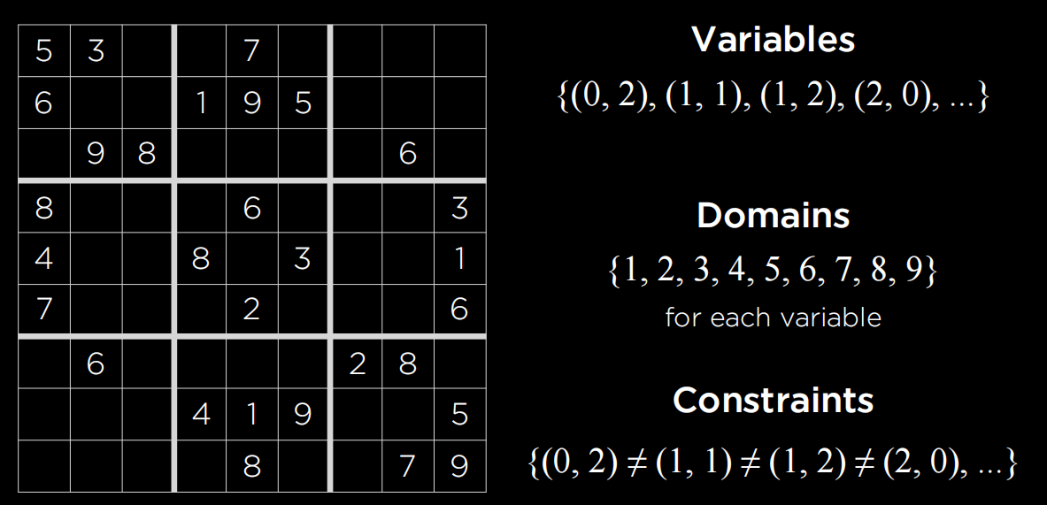
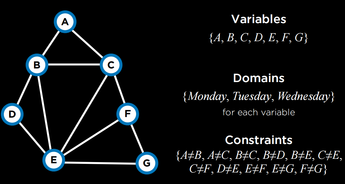
A few more terms worth knowing about constraint satisfaction problems:

• A Hard Constraint is a constraint that must be satisfied in a correct solution.
• A Soft Constraint is a constraint that expresses which solution is preferred over others.
• A Unary Constraint is a constraint that involves only one variable. In our example, a unary constraint would be saying that course A can’t have an exam on Monday {A ≠ Monday}.
• A Binary Constraint is a constraint that involves two variables. This is the type of constraint that we used in the example above, saying that some two courses can’t have the same value {A ≠ B}.

Node Consistency

Node consistency is when all the values in a variable’s domain satisfy the variable’s unary constraints.

Else we’ll remove something from the domain in order to satisfy the constraint.

Arc Consistency

Arc consistency is when all the values in a variable’s domain satisfy the variable’s binary constraints (note that we are now using “arc” to refer to what we previously referred to as “edge”). In other words, to make X arc-consistent with respect to Y, remove elements from X’s domain until every choice for X has a possible choice for Y.

When X choose any one in X’s domain, there is at least one choice that Y can choose in Y’s domain that satisfy Y’s constraint. If not, we need to remove something from X’s domain.

function Revise(csp, X, Y):

• revised = false
• for x in X.domain:
  • if no y in Y.domain satisfies constraint for (X,Y):
    • delete x from X.domain
    • revised = true
• return revised

Often we are interested in making the whole problem arc-consistent and not just one variable with respect to another. In this case, we will use an algorithm called AC-3, which uses Revise:

function AC-3(csp):

• queue = all arcs in csp
• while queue non-empty:
  • (X, Y) = Dequeue(queue)
  • if Revise(csp, X, Y):
    • if size of X.domain == 0:
      • return false
    • for each Z in X.neighbors - {Y}:
      • Enqueue(queue, (Z,X))
• return true

While the algorithm for arc consistency can simplify the problem, it will not necessarily solve it, since it considers binary constraints only and not how multiple nodes might be interconnected.

CSPs as Search Problems

• initial state: empty assignment (no variables)
• actions: add a {variable = value} to assignment
• transition model: shows how adding an assignment changes the assignment
• goal test: check if all variables assigned and constraints all satisfied
• path cost function: all paths have same cost

Backtracking Search

function Backtrack(assignment, csp):

• if assignment complete:
  • return assignment
• var = Select-Unassigned-Var(assignment, csp)
• for value in Domain-Values(var, assignment, csp):
  • if value consistent with assignment:
    • add {var = value} to assignment
    • result = Backtrack(assignment, csp)
    • if result ≠ failure:
      • return result
    • remove {var = value} from assignment
• return failure

Inference

maintaining arc-consistency

algorithm for enforcing arc-consistency every time we make a new assignment

When we make a new assignment to X, calls AC-3, starting with a queue of all arcs (Y, X)where Y is a neighbor of X

function Backtrack(assignment, csp):

• if assignment complete:
  • return assignment
• var = Select-Unassigned-Var(assignment, csp)
• for value in Domain-Values(var, assignment, csp):
  • if value consistent with assignment:
    • add {var = value} to assignment
    • inferences = Inference(assignment, csp)
    • if inferences ≠ failure:
      • add inferences to assignment
    • result = Backtrack(assignment, csp)
    • if result ≠ failure:
      • return result
    • remove {var = value} and inferences from assignment
• return failure

SELECT-UNASSIGNED-VAR

• minimum remaining values (MRV)** heuristic: select the variable that has the smallest domain
• degree heuristic: select the variable that has the highest degree

DOMAIN-VALUES

• least-constraining values heuristic: return variables in order by number of choices that are ruled out for neighboring variables
  • try least-constraining values first

Lecture 4 Learning

Machine Learning

Three categories : Supervised Learning, Reinforcement Learning and Unsupervised Learning.

1) Supervised Learning

given a data set of input-output pairs, learn a function to map inputs to outputs

Classification

supervised learning task of learning a function mapping an input point to a discrete category

There are lots of ways to classify:

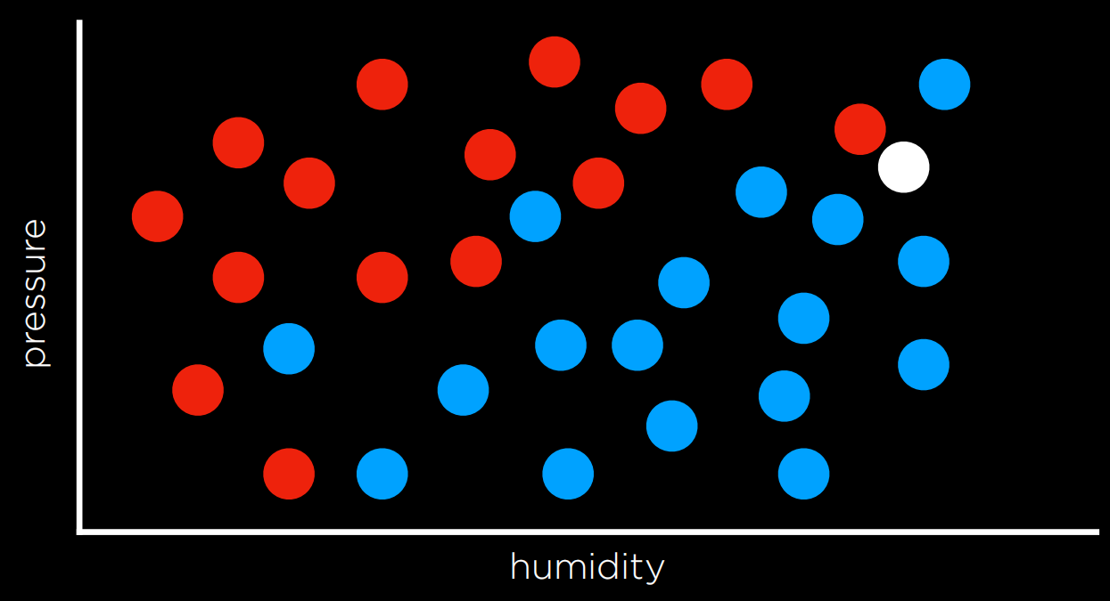
1. k-nearest-neighbor classification

algorithm that, given an input, chooses the most common class out of the k nearest data points to that input

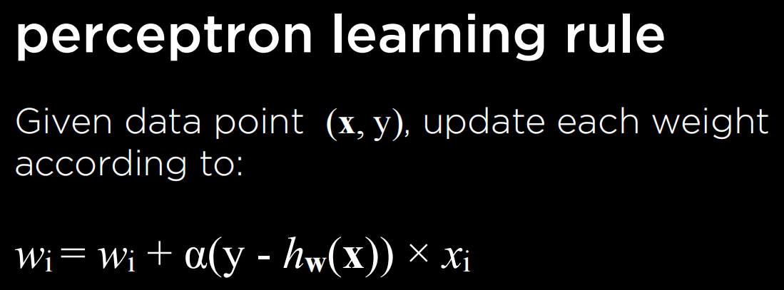
2. Perceptron Learning

Another way of going about a classification problem, as opposed to the nearest-neighbor strategy, is looking at the data as a whole and trying to create a decision boundary.

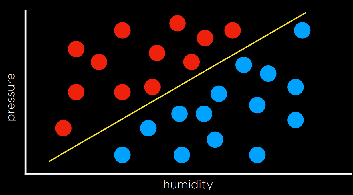
Goal:

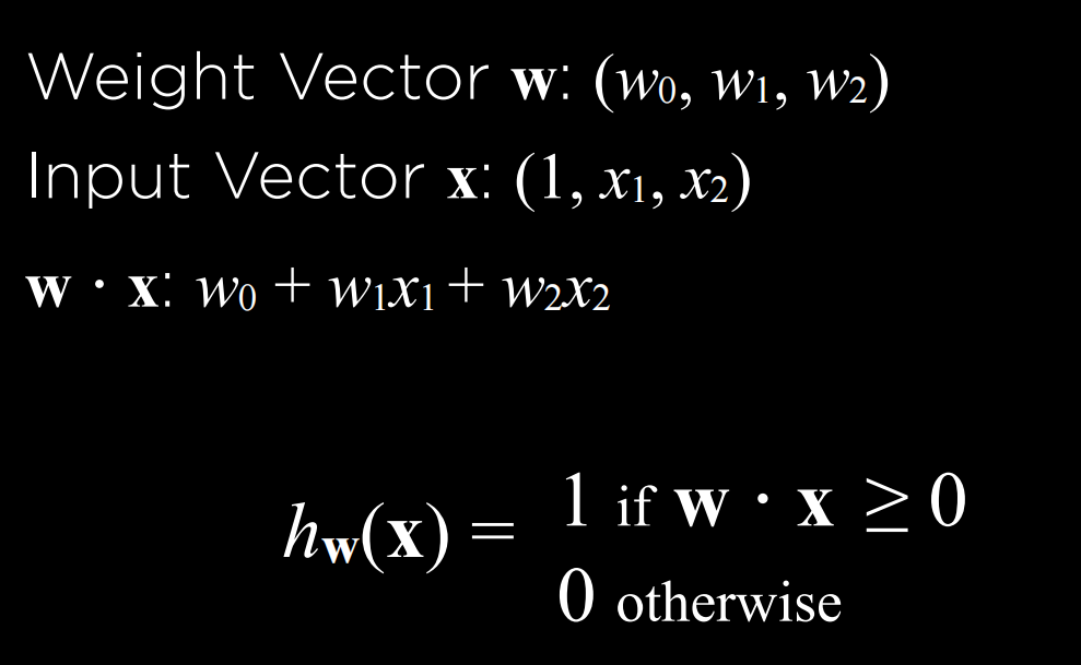
Learning Rule:

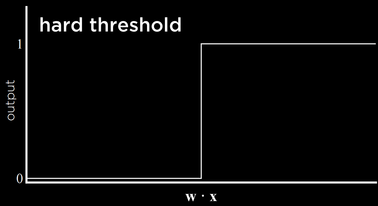
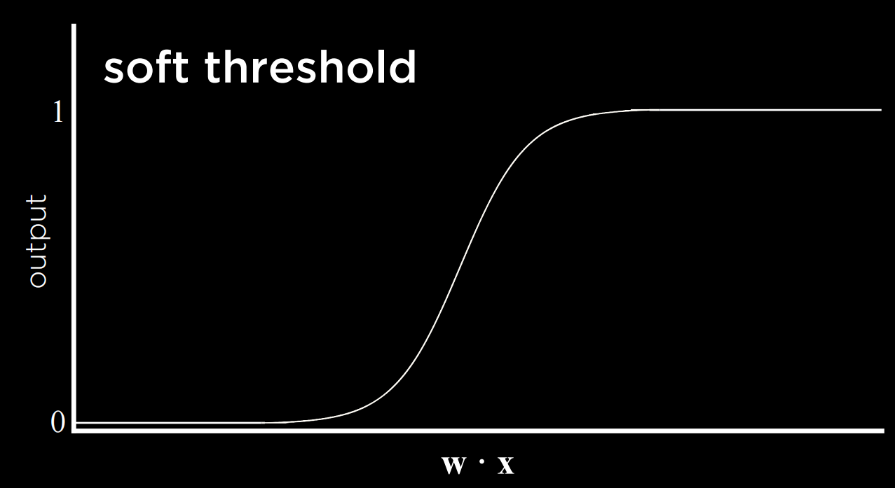
The problem with this type of function is that it is unable to express uncertainty, since it can only be equal to 0 or to 1. It employs a hard threshold. A way to go around this is by using a logistic function, which employs a soft threshold. A logistic function can yield a real number between 0 and 1, which will express confidence in the estimate. The closer the value to 1, the more likely it is to rain.

3. Support Vector Machines

Trying to find

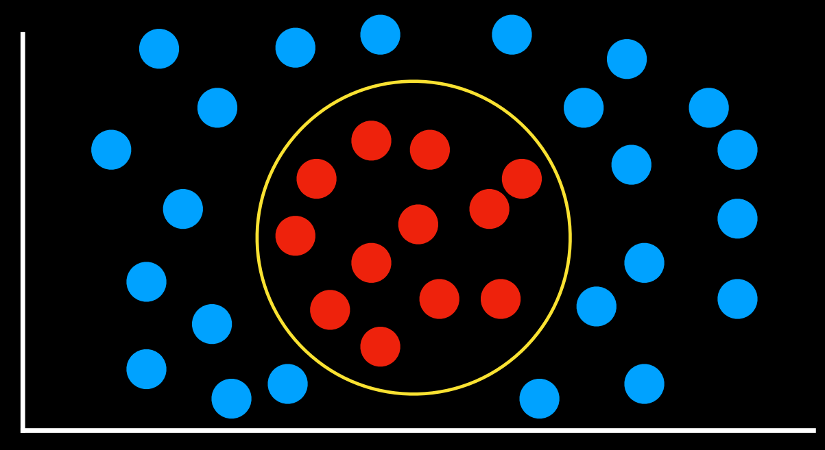
maximum margin separator

boundary that maximizes the distance between any of the data points

It can be non-linear.

Regression

supervised learning task of learning a function mapping an input point to a continuous value

Loss function

function that expresses how poorly our hypothesis performs

For classification problems, we can use a 0-1 Loss Function.

• L(actual, predicted):
  • 0 if actual = predicted
  • 1 otherwise

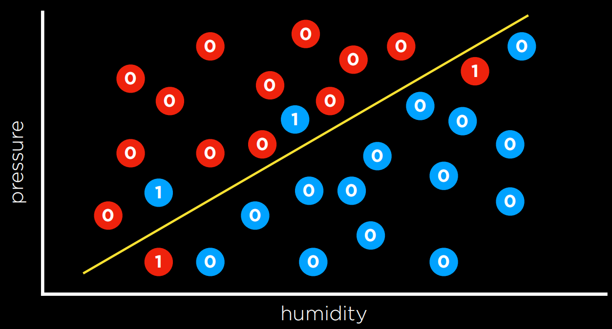
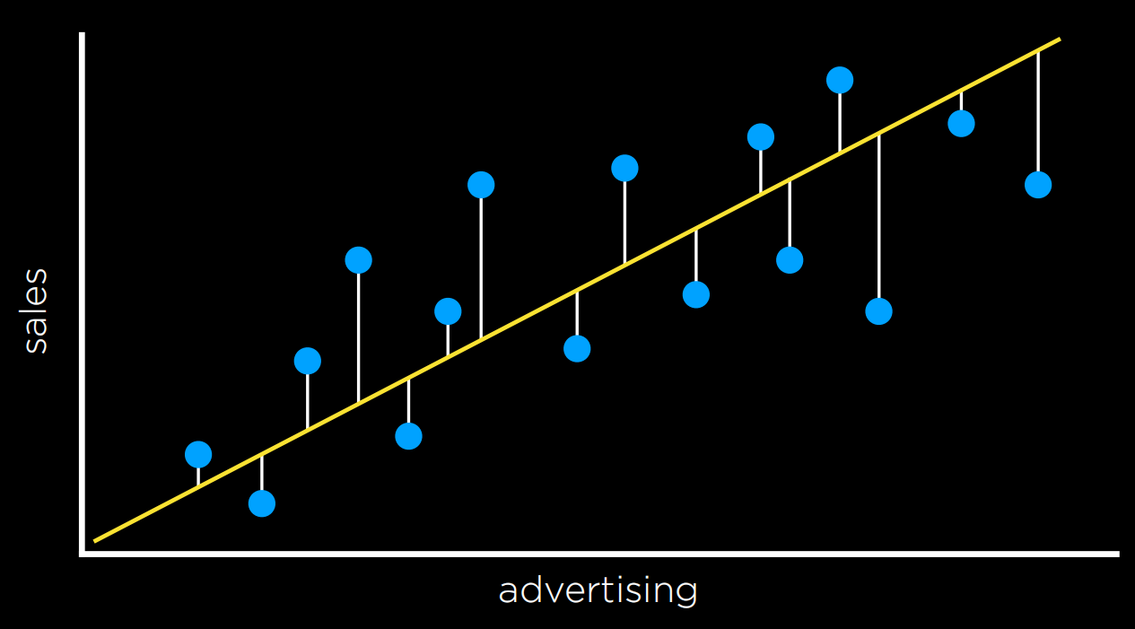
L₁ and L₂ loss functions can be used when predicting a continuous value. In this case, we are interested in quantifying for each prediction how much it differed from the observed value. We do this by taking either the absolute value or the squared value of the observed value minus the predicted value (i.e. how far the prediction was from the observed value).

• L₁: L(actual, predicted) = |actual - predicted|
• L₂: L(actual, predicted) = (actual - predicted)²

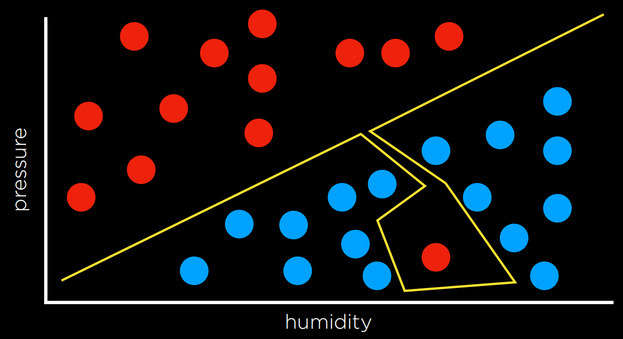
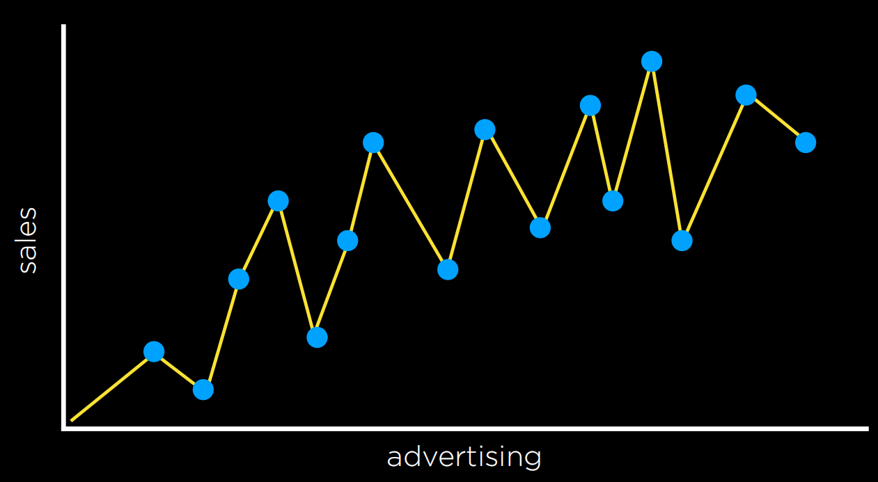
Overfitting

a model that fits too closely to a particular data set and therefore may fail to generalize to future data

Regularization

penalizing hypotheses that are more complex to favor simpler, more general hypotheses

cost(h) = loss(h) + λcomplexity(h)

If the model is too complex, like the two graphs up there, we should give some penalty to avoid overfitting.

holdout cross-validation

splitting data into a training set and a test set, such that learning happens on the training set and is evaluated on the test set

k-fold cross-validation

splitting data into k sets, and experimenting k times, using each set as a test set once, and using remaining data as training set

scikit-learn

As often is the case with Python, there are multiple libraries that allow us to conveniently use machine learning algorithms. One of such libraries is scikit-learn.

2) Reinforcement Learning

given a set of rewards or punishments, learn what actions to take in the future

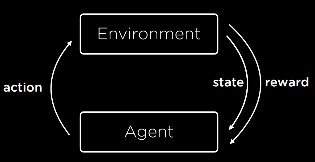
Markov Decision Process

model for decision-making, representing states, actions, and their rewards

Reinforcement learning can be viewed as a Markov decision process, having the following properties:

• Set of states S
• Set of actions Actions(S)
• Transition model P(s’ | s, a)
• Reward function R(s, a, s’)

Q-learning

one model of reinforcement learning, where a function Q(s, a) outputs an estimate of the value of taking action a in state s.

The model starts with all estimated values equal to 0 (Q(s,a) = 0 for all s, a). When an action is taken and a reward is received, the function does two things: 1) it estimates the value of Q(s, a) based on current reward and expected future rewards, and 2) updates Q(s, a) to take into account both the old estimate and the new estimate. This gives us an algorithm that is capable of improving upon its past knowledge without starting from scratch.

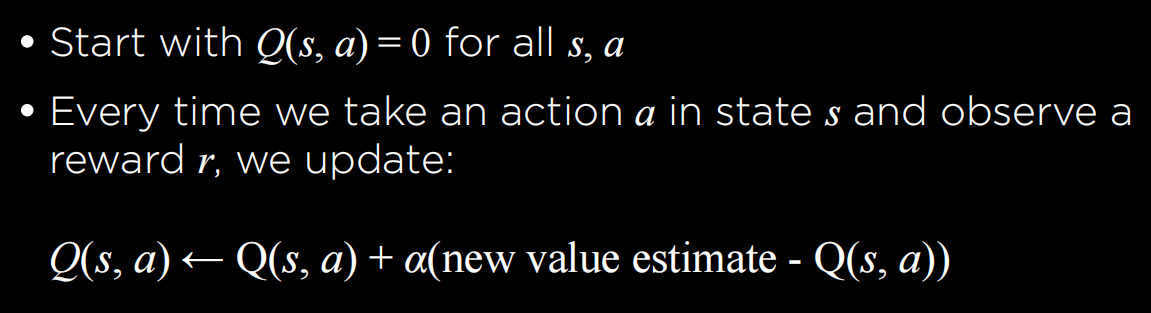
$\alpha$ : learning rate, represent how much we value new information compared to old information.

r is the reward of this step. What’s more, we can add some future rewards into it:

For example:

Or:

Greedy Decision-Making

When in state s, choose action a with highest Q(s, a)

This brings us to discuss the Explore vs. Exploit tradeoff. A greedy algorithm always exploits, taking the actions that are already established to bring to good outcomes. However, it will always follow the same path to the solution, never finding a better path.

ε-greedy

• Set ε equal to how often we want to move randomly.
• With probability 1 - ε, choose estimated best move.
• With probability ε, choose a random move

function approximation

approximating Q(s, a), often by a function combining various features, rather than storing one value for every state-action pair

3) unsupervised learning

given input data without any additional feedback, learn patterns

clustering

organizing a set of objects into groups in such a way that similar objects tend to be in the same group

k-means clustering

algorithm for clustering data based on repeatedly assigning points to clusters and updating those clusters’ centers

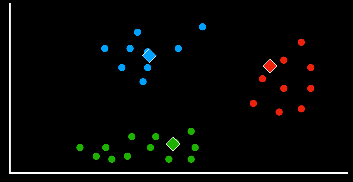
Set k centers. Divide all the data for these clusters. Move these centers lots of time.

Lecture 5 Neural Networks

Neural Networks

• Neurons are connected to and receive electrical signals from other neurons.
• Neurons process input signals and can be activated

Artificial Neural Networks

• Model mathematical function from inputs to outputs based on the structure and parameters of the network.
• Allows for learning the network’s parameters based on data.

When implemented in AI, the parallel of each neuron is a unit that’s connected to other units. For example, like in the last lecture, the AI might map two inputs, x₁ and x₂, to whether it is going to rain today or not. Last lecture, we suggested the following form for this hypothesis function: h(x₁, x₂) = w₀ + w₁x₁ + w₂x₂, where w₁ and w₂ are weights that modify the inputs, and w₀ is a constant, also called bias, modifying the value of the whole expression.

Activation Function

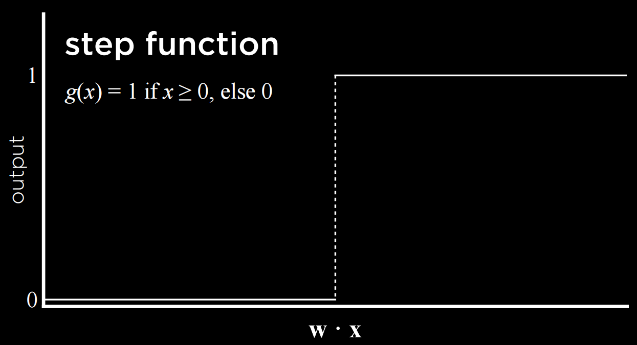
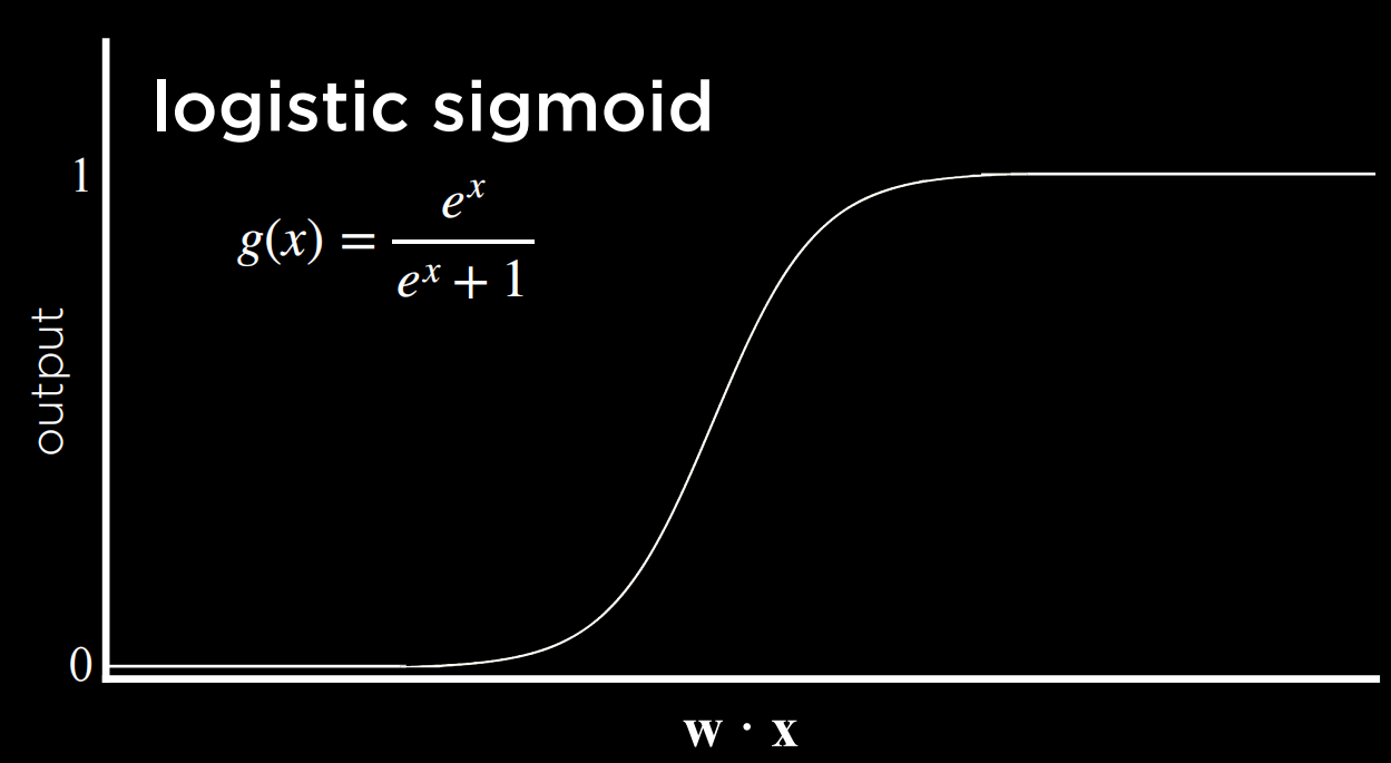
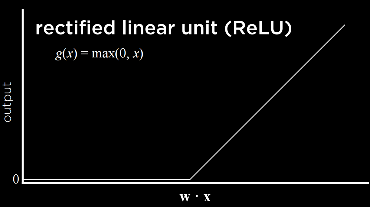
Neural Network Structure

Or logical connective can be presented as:

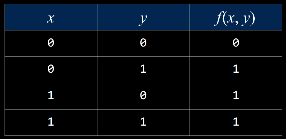
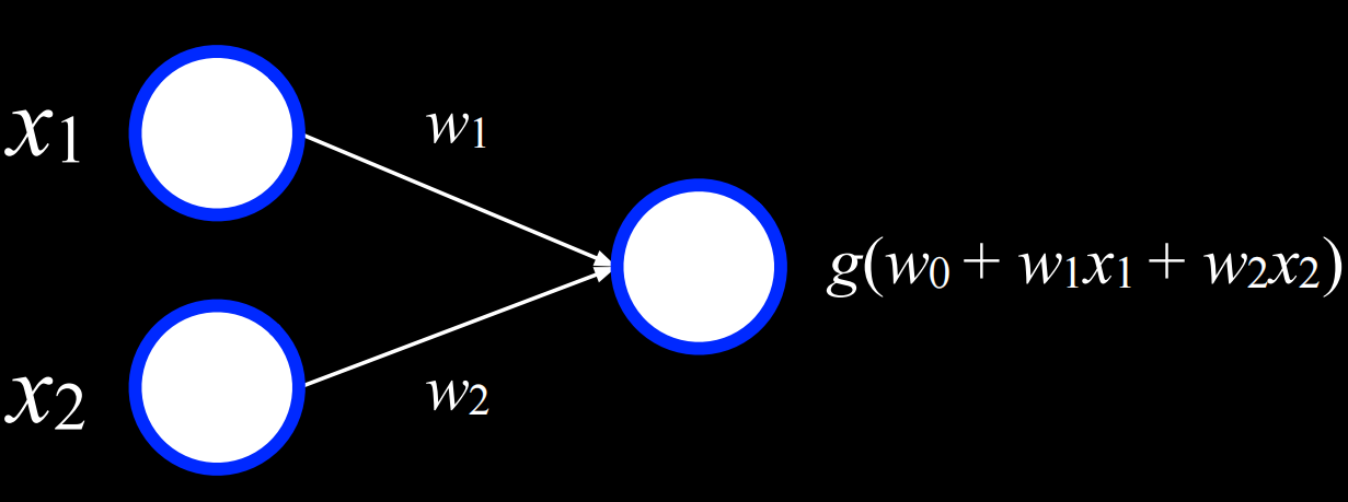
We can visualize this function as a neural network. x₁ is one input unit, and x₂ is another input unit. They are connected to the output unit by an edge with a weight of 1. The output unit then uses function g(-1 + 1x₁ + 2x₂) with a threshold of 0 to output either 0 or 1 (false or true).

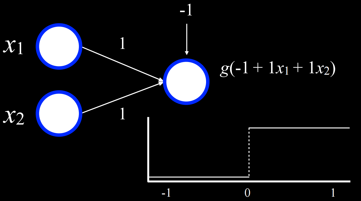
A similar process can be repeated with the And function (where the bias will be (-2)). Moreover, inputs and outputs don’t have to be distinct. A similar process can be used to take humidity and air pressure as input, and produce the probability of rain as output.

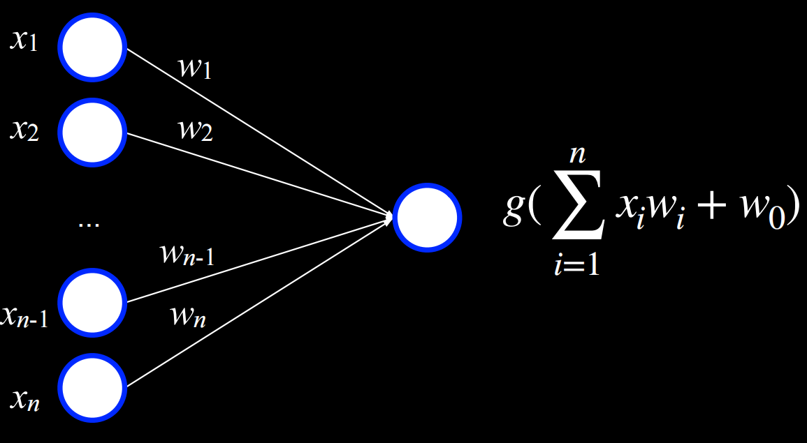
Gradient Descent

algorithm for minimizing loss when training neural network

• Start with a random choice of weights. This is our naive starting place, where we don’t know how much we should weight each input.
• Repeat:
  • Calculate the gradient based on all data points that will lead to decreasing loss. Ultimately, the gradient is a vector (a sequence of numbers).
  • Update weights according to the gradient.

Stochastic Gradient Descent: Calculate the gradient based on one data point

Mini-Batch Gradient Descent: Calculate the gradient based on one small batch

This can be done with any number of inputs and outputs, where each input is connected to each output, and where the outputs represent decisions that we can make. Note that in this kind of neural networks the outputs are not connected. These output has no relation, mens that we can construct neural network one by one.

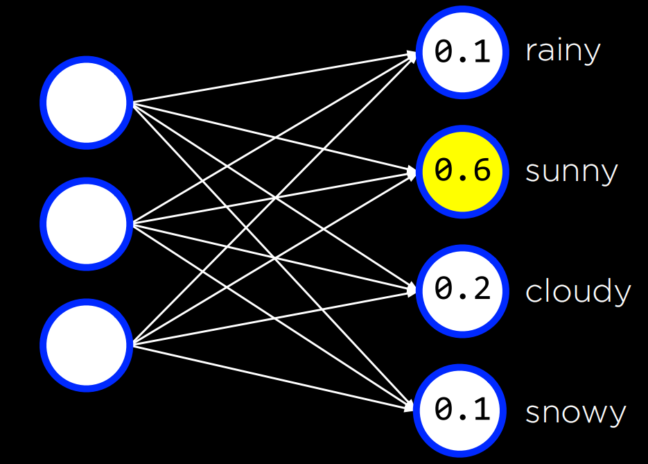
So far, our neural networks relied on perceptron output units. These are units that are only capable of learning a linear decision boundary, using a straight line to separate data. That is, based on a linear equation, the perceptron could classify an input to be one type or another (e.g. left picture). However, often, data are not linearly separable (e.g. right picture). In this case, we turn to multilayer neural networks to model data non-linearly.

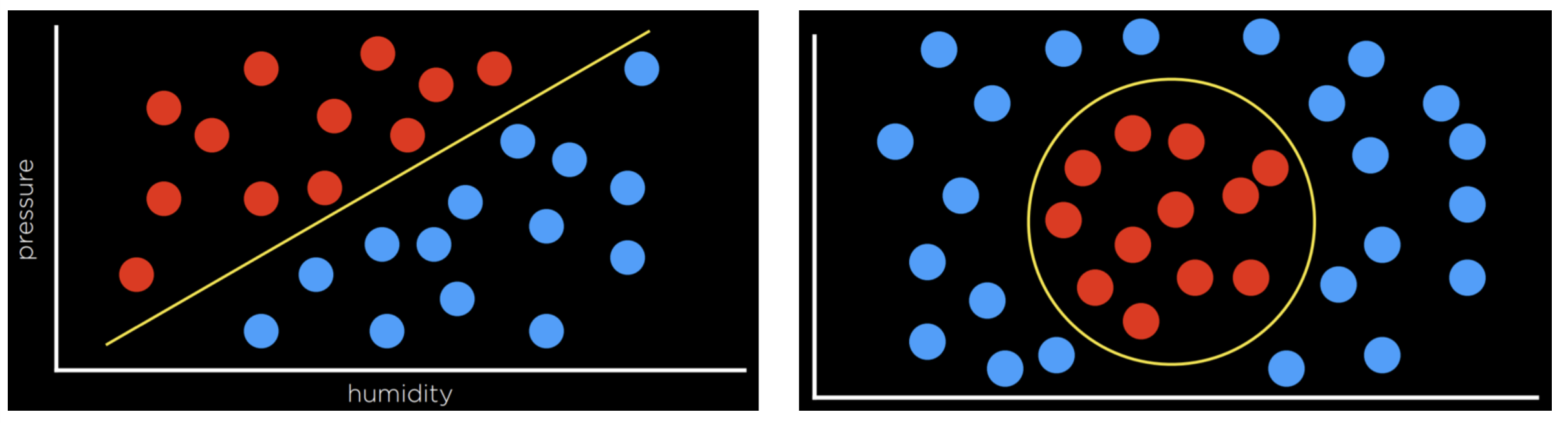
Multilayer Neural Networks

artificial neural network with an input layer, an output layer, and at least one hidden layer

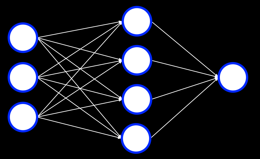
Backpropagation

algorithm for training neural networks with hidden layers

• Calculate error for output layer
• For each layer, starting with output layer and moving inwards towards earliest hidden layer:
  • Propagate error back one layer. In other words, the current layer that’s being considered sends the errors to the preceding layer.
  • Update weights.

This can be extended to any number of hidden layers, creating deep neural networks, which are neural networks that have more than one hidden layer.

Overfitting

dropout

temporarily removing units — selected at random — from a neural network to prevent over-reliance on certain units

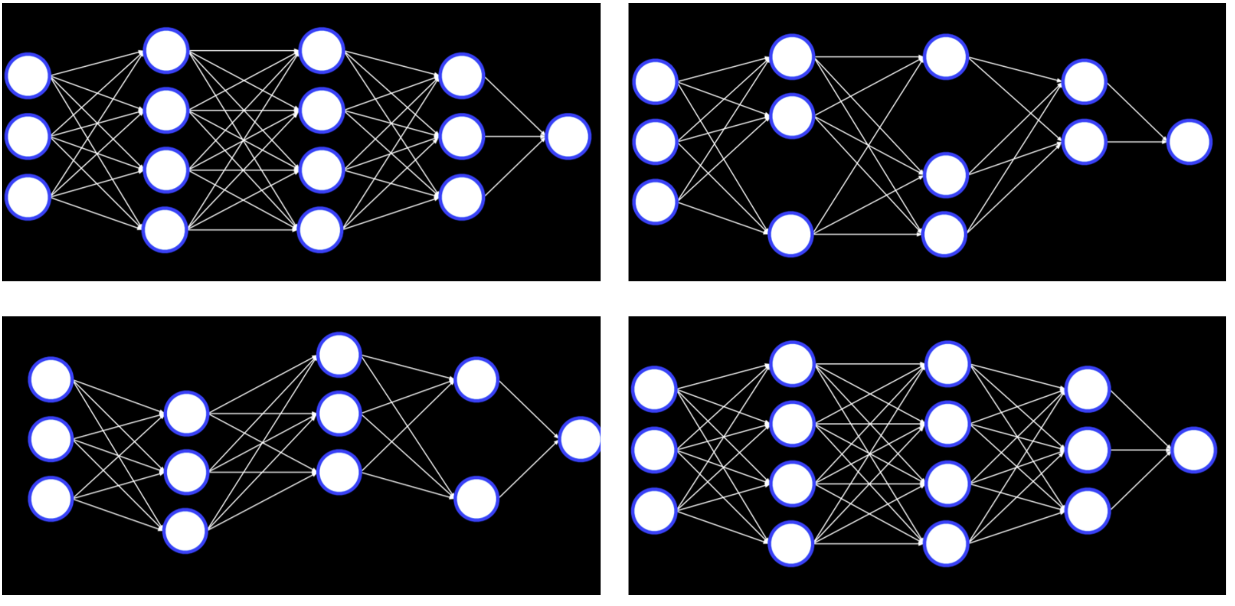
Note that after the training is finished, the whole neural network will be used again.

TensorFlow

You can experiment with TensorFlow neural networks in this web application

computer vision

computational methods for analyzing and understanding digital images

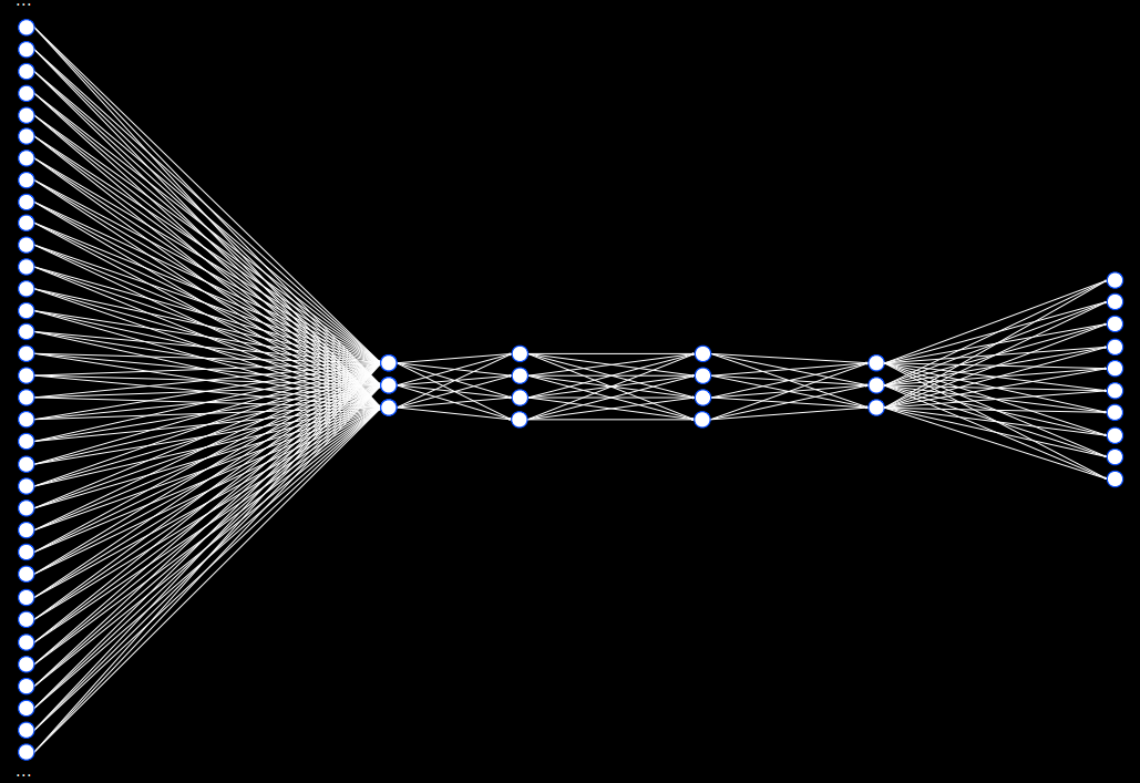
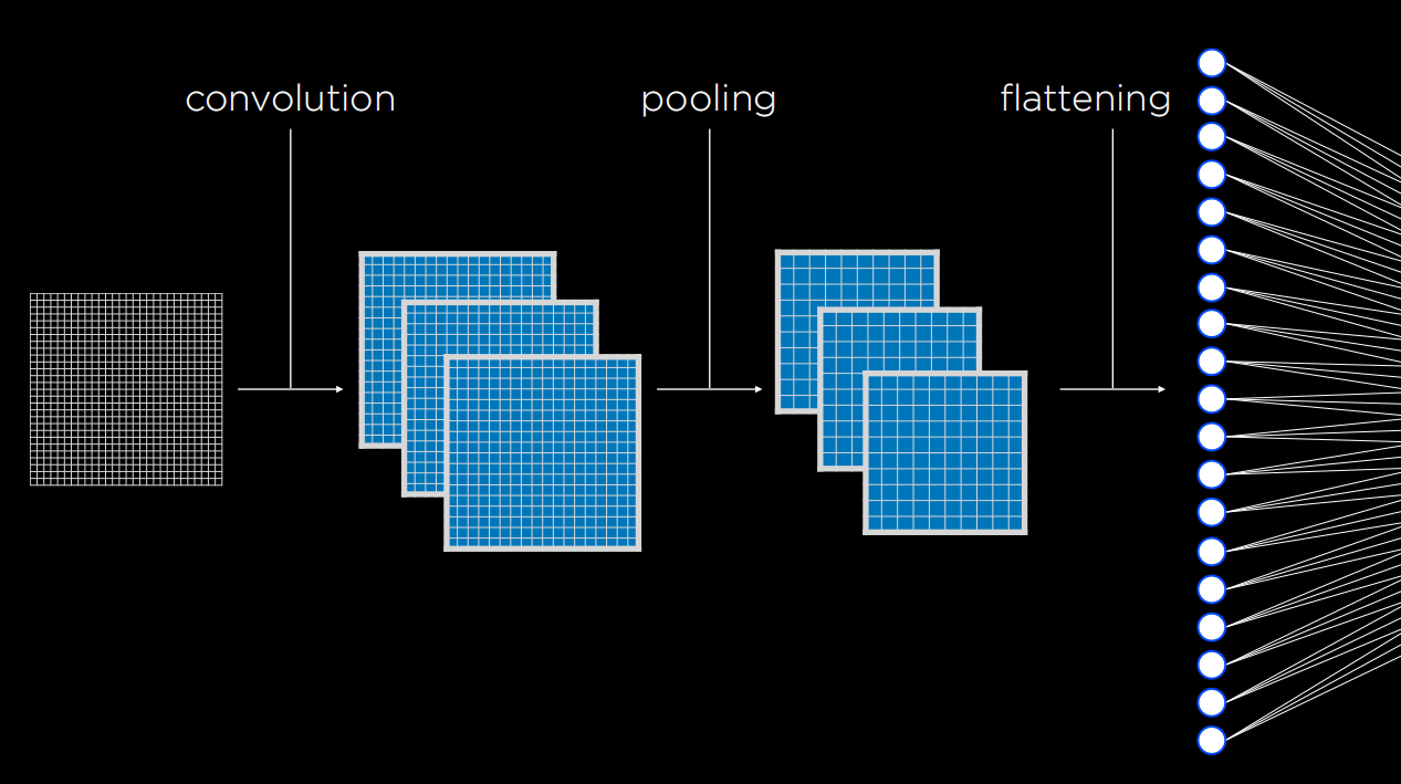
Images consist of pixels, and pixels are represented by three values that range from 0 to 255, one for red, one for green and one for blue. These values are often referred to with the acronym RGB. We can use this to create a neural network where each color value in each pixel is an input, where we have some hidden layers, and the output is some number of units that tell us what it is that was shown in the image. However, there are a few drawbacks to this approach. First, by breaking down the image into pixels and the values of their colors, we can’t use the structure of the image as an aid. That is, as humans, if we see a part of a face we know to expect to see the rest of the face, and this quickens computation. We want to be able to use a similar advantage in our neural networks. Second, the sheer number of inputs is very big, which means that we will have to calculate a lot of weights.

Image Convolution

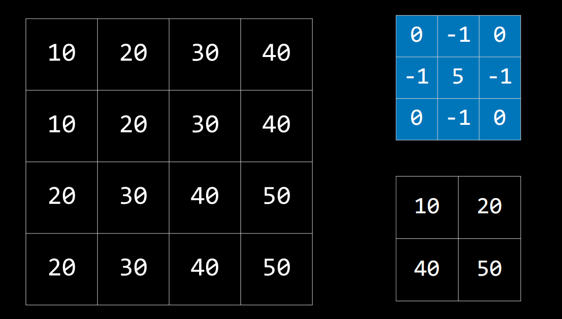
applying a filter that adds each pixel value of an image to its neighbors, weighted according to a kernel matrix

The kernel is the blue matrix, and the image is the big matrix on the left. The resulting filtered image is the small matrix on the bottom right. To filter the image with the kernel, we start with the pixel with value 20 in the top-left of the image (coordinates 1,1). Then, we will multiply all the values around it by the corresponding value in the kernel and sum them up (100 + 20(-1) + 300 + 10(-1) + 205 + 30(-1) + 200 + 30(-1) + 40*0), producing the value 10.

Different kernels can achieve different tasks. For edge detection, the following kernel is often used:

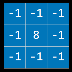
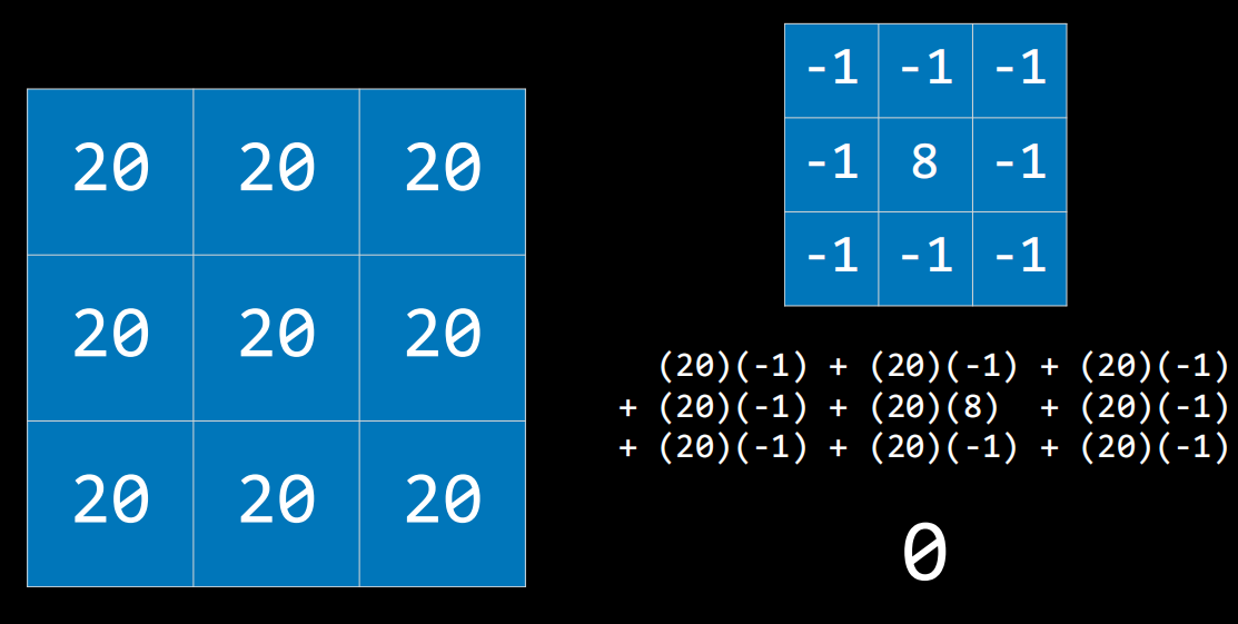
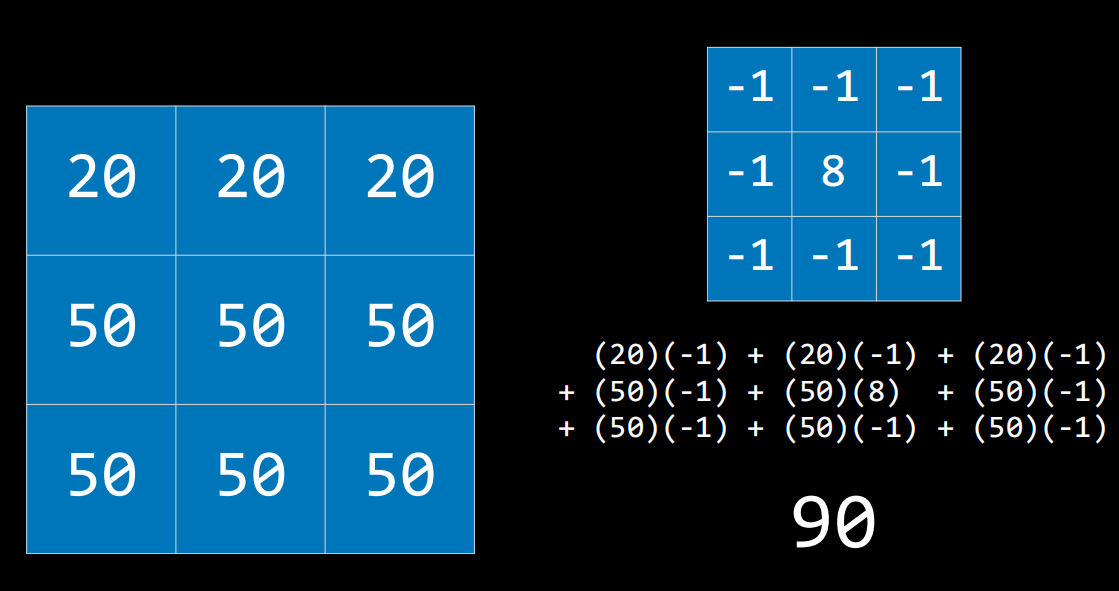
The idea here is that when the pixel is similar to all its neighbors, they should cancel each other, giving a value of 0. Therefore, the more similar the pixels, the darker the part of the image, and the more different they are the lighter it is. Applying this kernel to an image (left) results in an image with pronounced edges (right):

We can use the PIL library (stands for Python Imaging Library) that can do most of the hard work for us.

Still, processing the image in a neural network is computationally expensive due to the number of pixels that serve as input to the neural network.

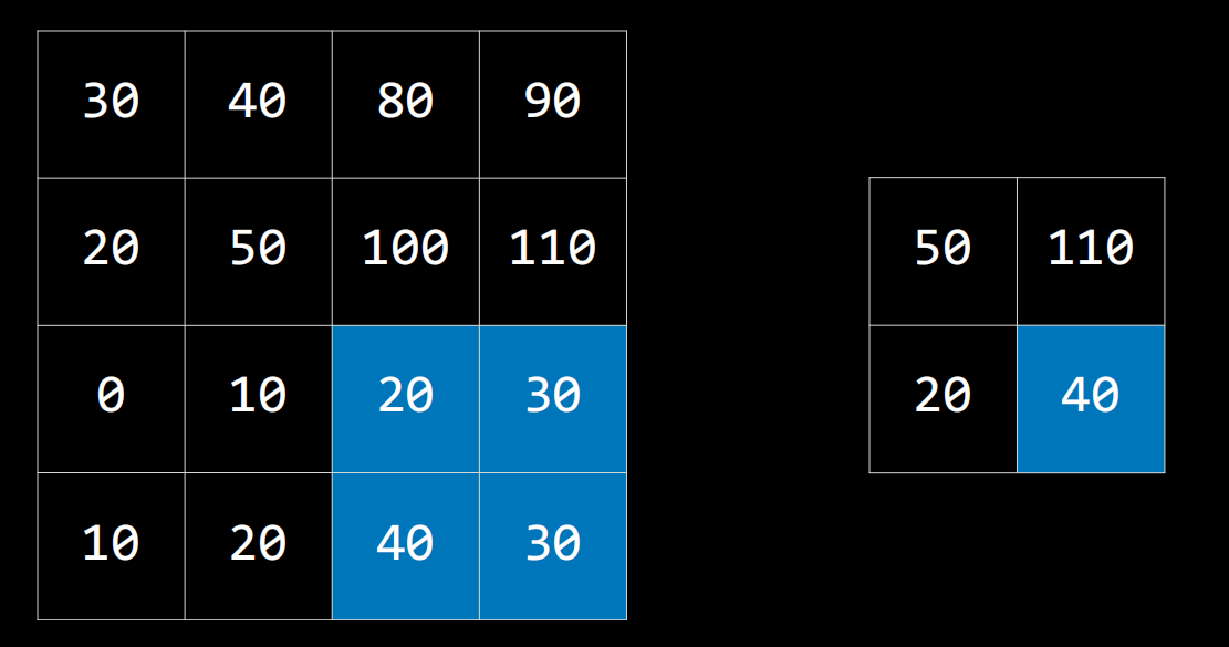
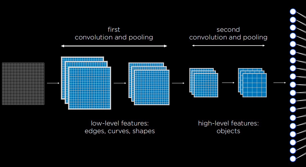
pooling

reducing the size of an input by sampling from regions in the input

max-pooling

pooling by choosing the maximum value in each region

convolutional neural network

neural networks that use convolution, usually for analyzing images

Recurrent Neural Networks

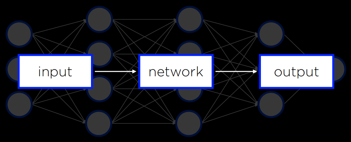
feed-forward neural network

neural network that has connections only in one direction

Feed-Forward Neural Networks are the type of neural networks that we have discussed so far, where input data is provided to the network, which eventually produces some output. A diagram of how feed-forward neural networks work can be seen below.

recurrent neural network

neural network that generates output that feeds back into its own inputs

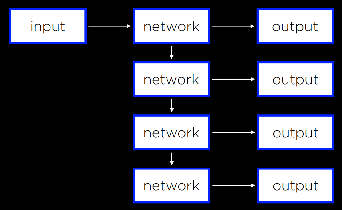
As opposed to that, Recurrent Neural Networks consist of a non-linear structure, where the network uses its own output as input. For example, Microsoft’s captionbot is capable of describing the content of an image with words in a sentence.

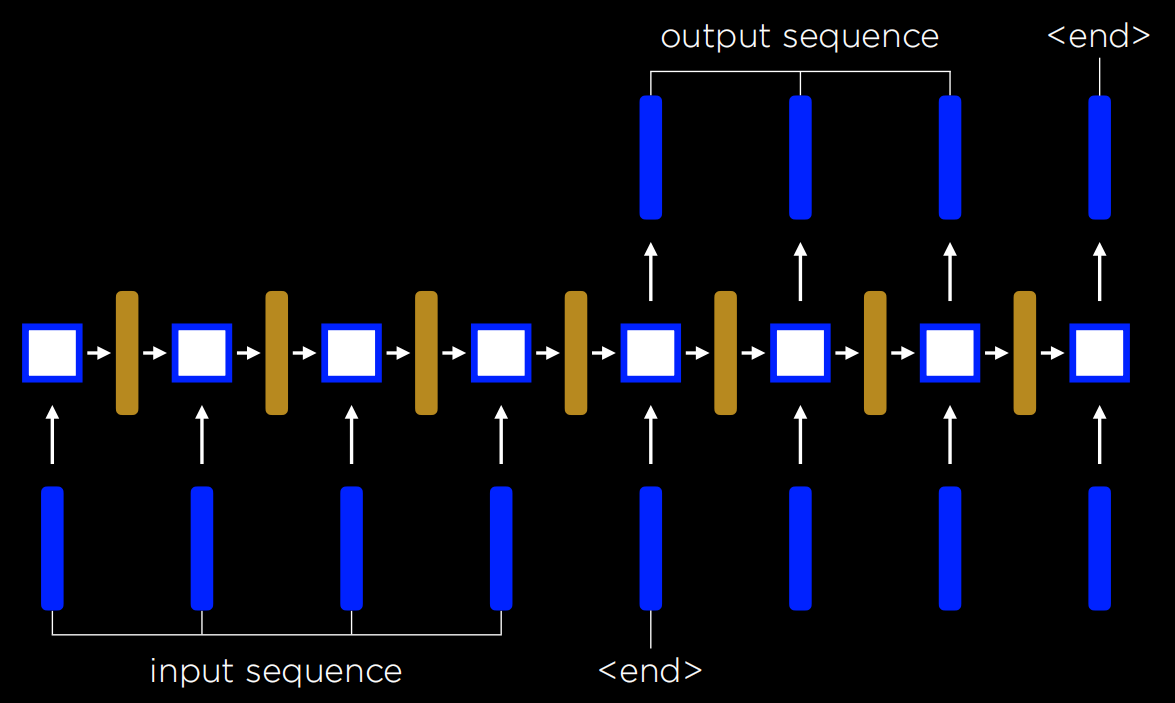
Recurrent neural networks are helpful in cases where the network deals with sequences and not a single individual object. Above, the neural network needed to produce a sequence of words. However, the same principle can be applied to analyzing video files, which consist of a sequence of images, or in translation tasks, where a sequence of inputs (words in the source language) is processed to produce a sequence of outputs (words in the target language).

Video analysis:

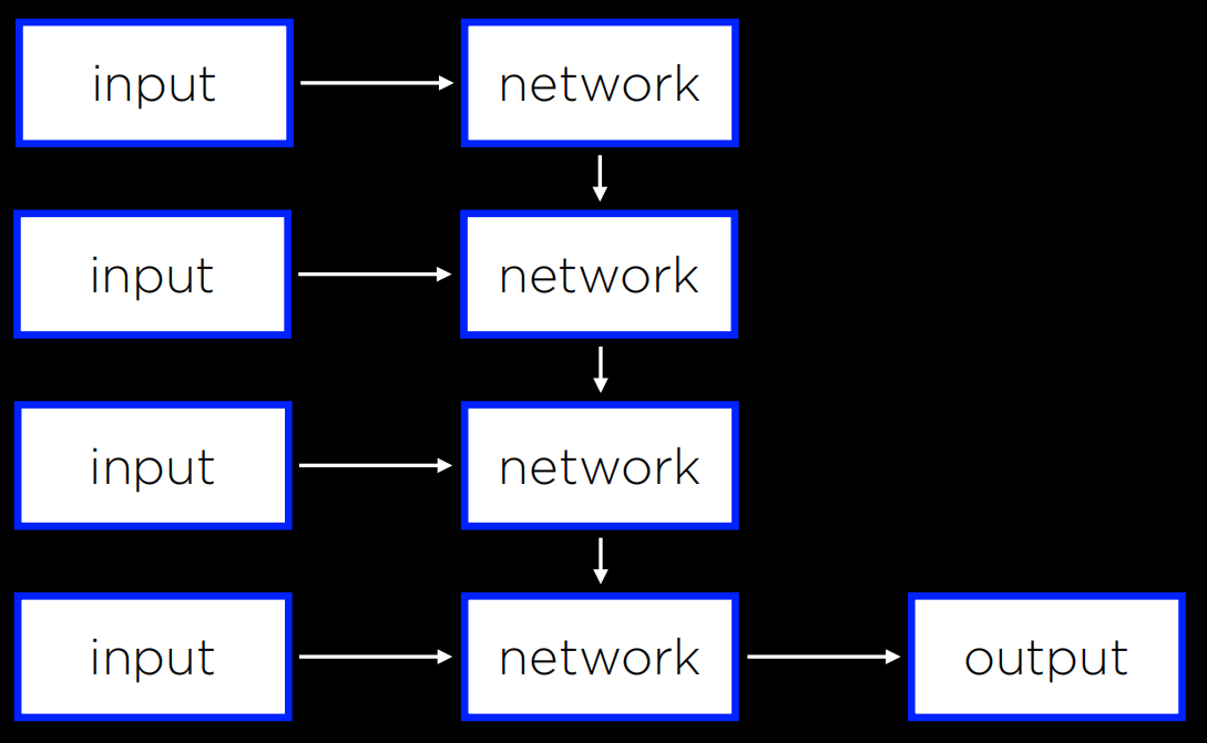
Translation:

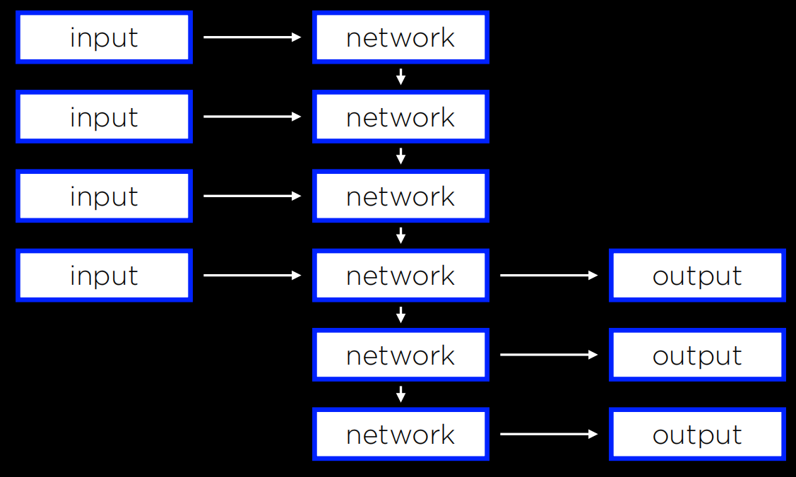
Lecture 6 Language

Language

Natural Language Processing spans all tasks where the AI gets human language as input. The following are a few examples of such tasks:

• automatic summarization, where the AI is given text as input and it produces a summary of the text as output.
• information extraction, where the AI is given a corpus of text and the AI extracts data as output.
• language identification, where the AI is given text and returns the language of the text as output.
• machine translation, where the AI is given a text in the origin language and it outputs the translation in the target language.
• named entity recognition, where the AI is given text and it extracts the names of the entities in the text (for example, names of companies).
• speech recognition, where the AI is given speech and it produces the same words in text.
• text classification, where the AI is given text and it needs to classify it as some type of text.
• word sense disambiguation, where the AI needs to choose the right meaning of a word that has multiple meanings (e.g. bank means both a financial institution and the ground on the sides of a river).

Syntax and Semantics

Context-Free Grammar

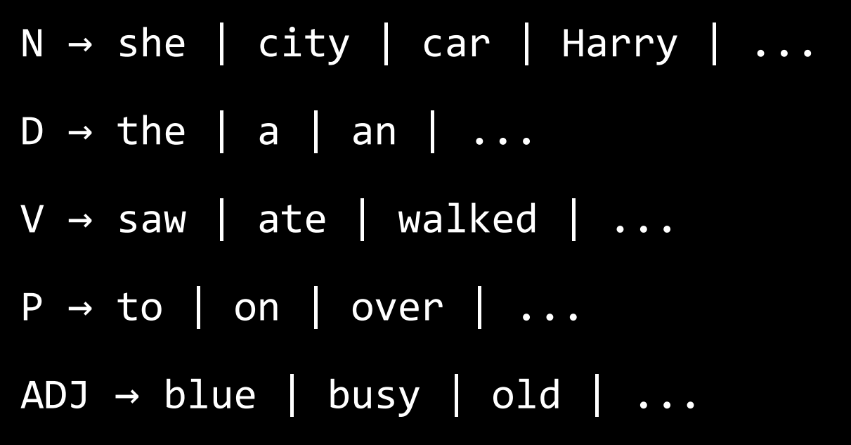
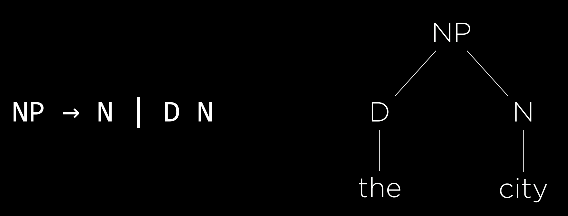
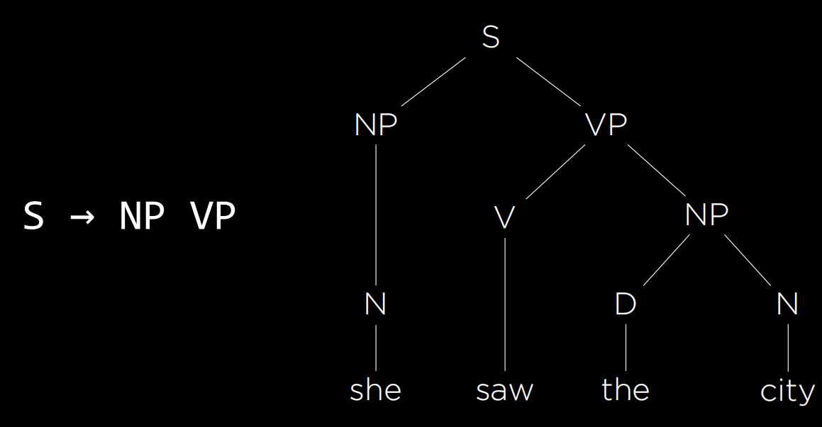
nltk

n-grams

a contiguous sequence of n items from a sample of text

Tokenization

the task of splitting a sequence of

characters into pieces (tokens)

Markov Models

As discussed in previous lectures, Markov models consist of nodes, the value of each of which has a probability distribution based on a finite number of previous nodes. Markov models can be used to generate text. To do so, we train the model on a text, and then establish probabilities for every n-th token in an n-gram based on the n words preceding it. For example, using trigrams, after the Markov model has two words, it can choose a third one from a probability distribution based on the first two. Then, it can choose a fourth word from a probability distribution based on the second and third words.

Bag-of-words model

model that represents text as an unordered collection of words

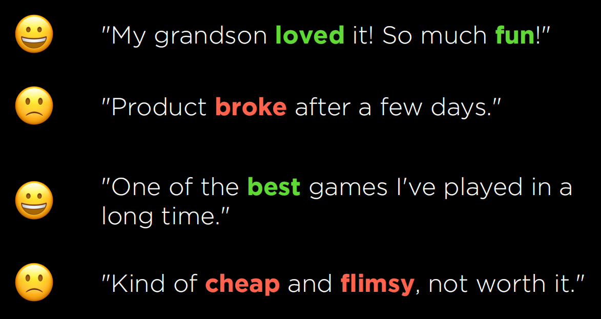
Naive Bayes

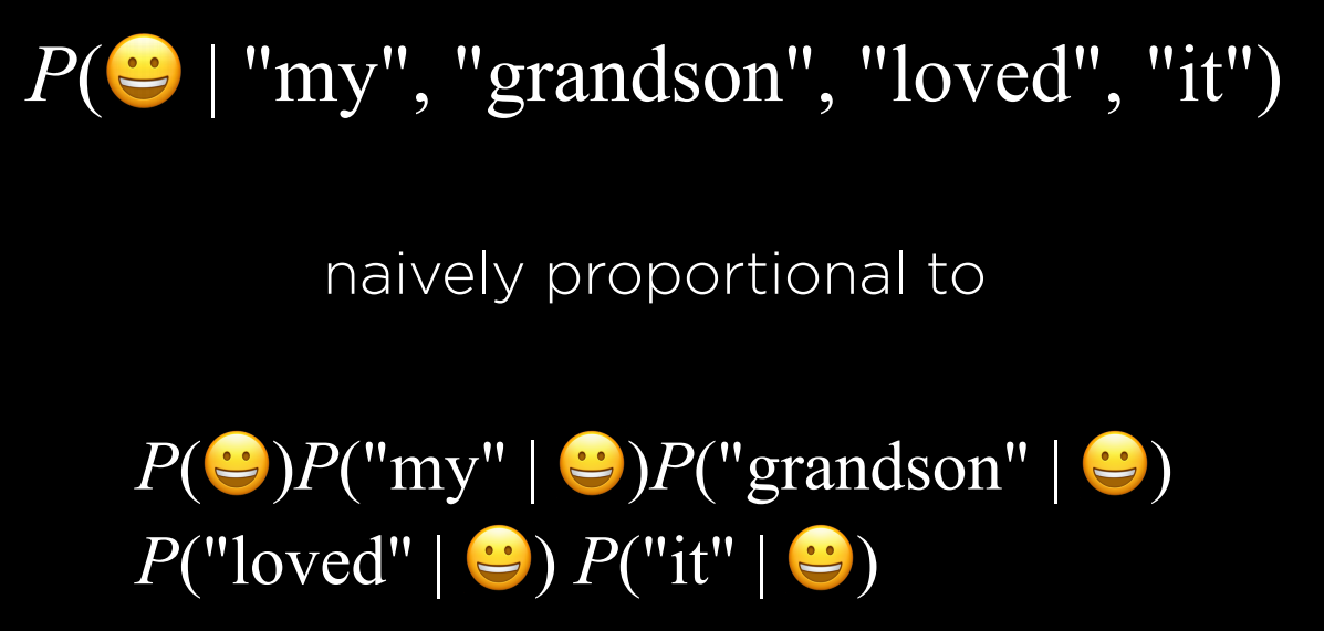
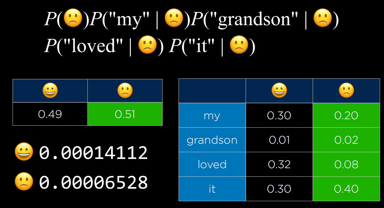
additive smoothing

adding a value α to each value in our distribution to smooth the data

Laplace smoothing

adding 1 to each value in our distribution: pretending we’ve seen each value one more time than we actually have

Word Representation

one-hot representation

representation of meaning as a vector with a single 1, and with other values as 0

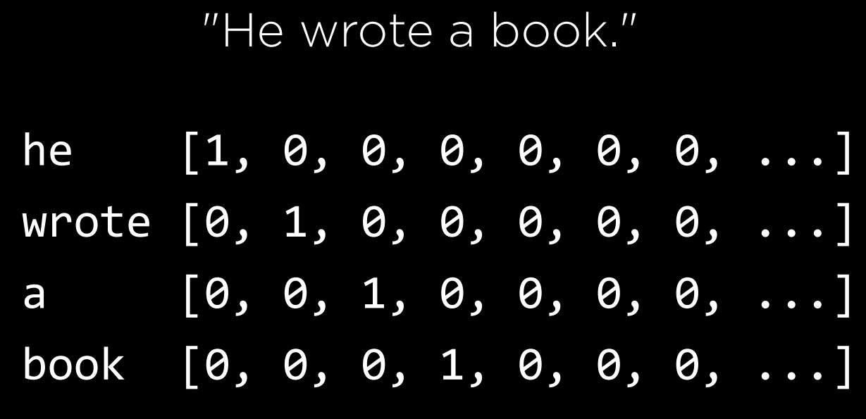
However, while this representation works in a world with four words, if we want to represent words from a dictionary, when we can have 50,000 words, we will end up with 50,000 vectors of length 50,000. This is incredibly inefficient. Another problem in this kind of representation is that we are unable to represent similarity between words like “wrote” and “authored.”

distributed representation

representation of meaning distributed across multiple values

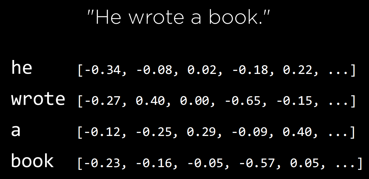
word2vec

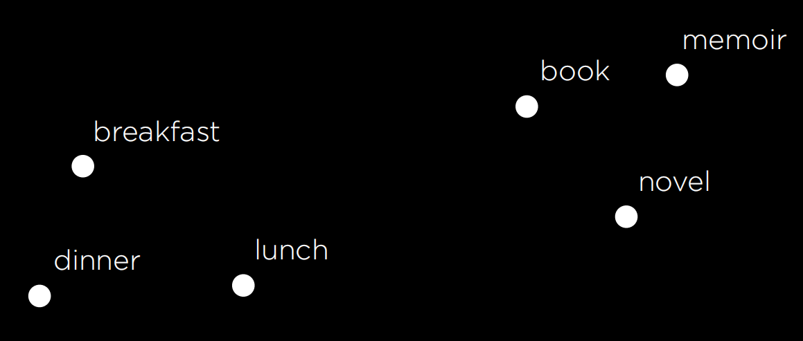
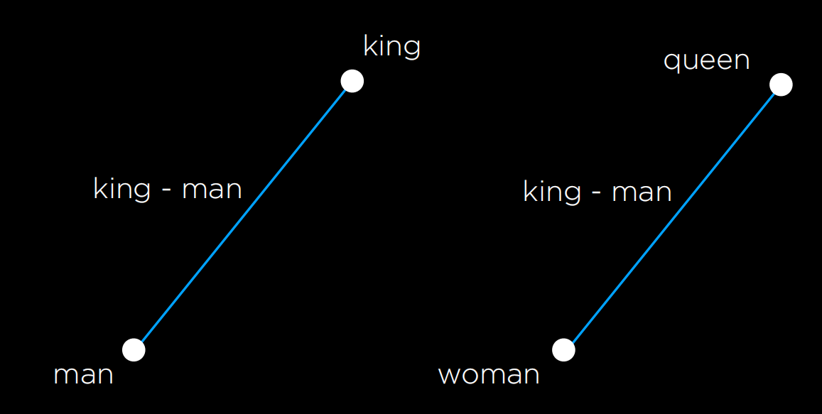
word2vec is an algorithm for generating distributed representations of words. It does so by Skip-Gram Architecture, which is a neural network architecture for predicting context given a target word.

Neural Networks

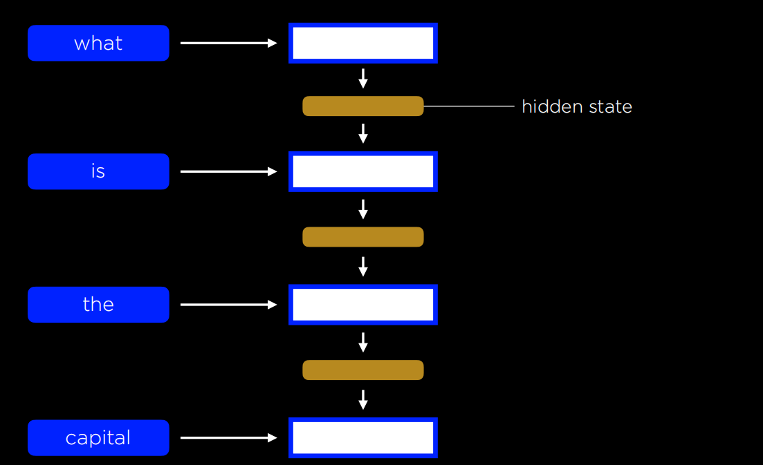
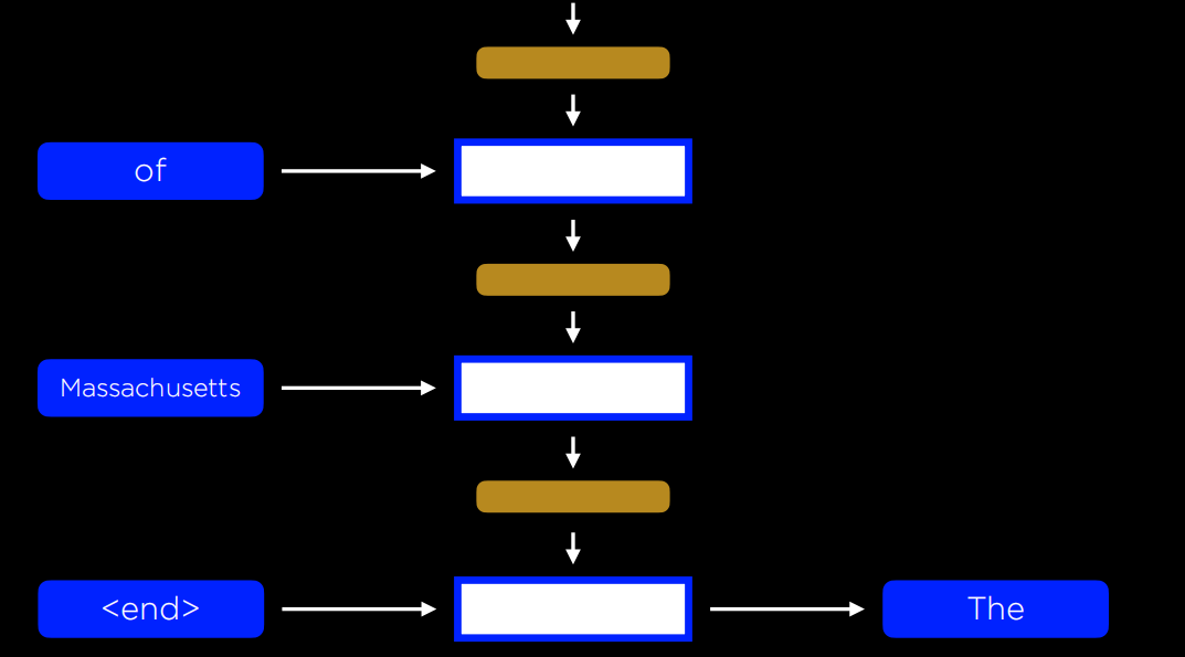
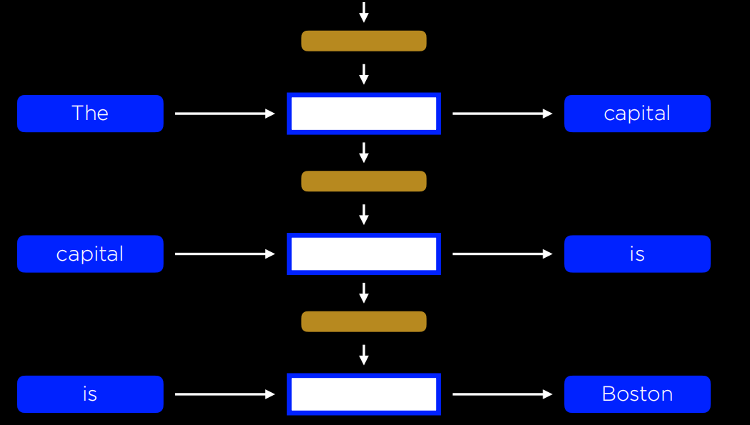
We use Recurrent neural networks :

Attention

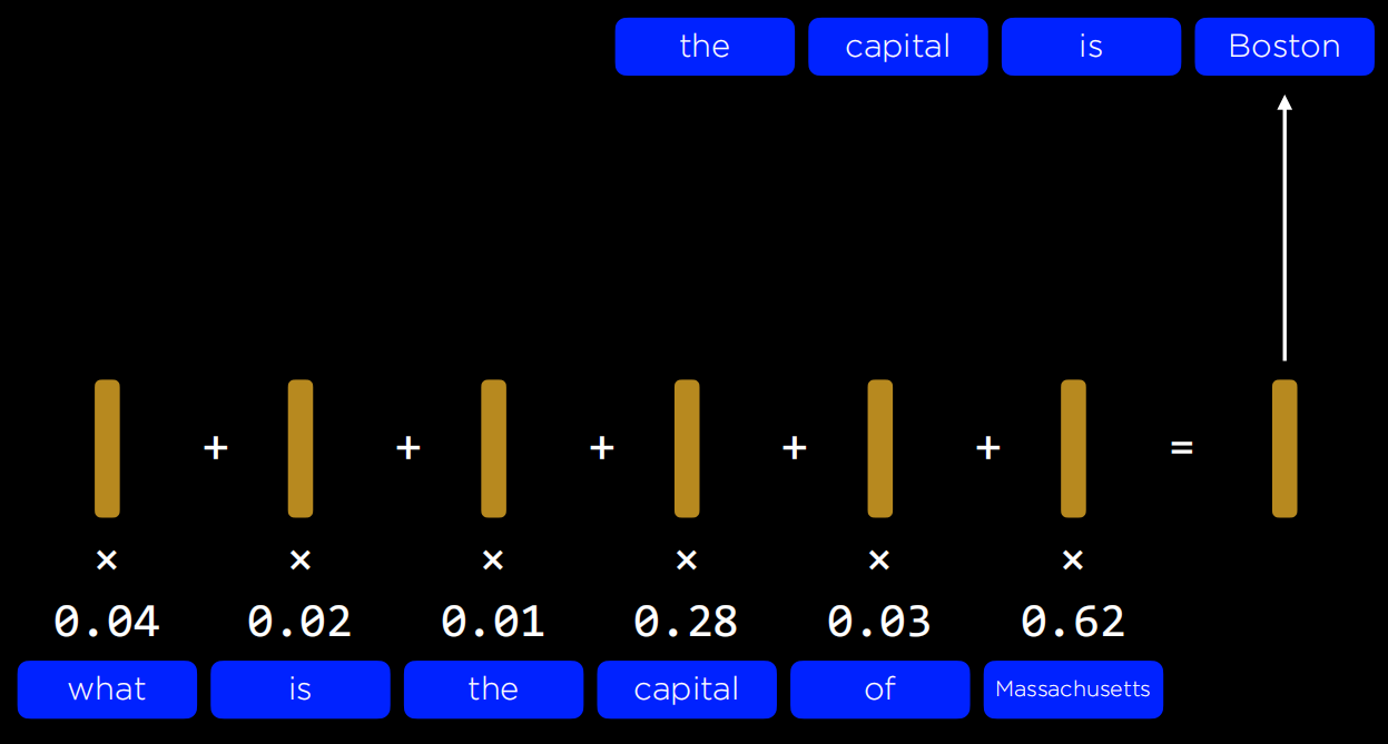
Attention refers to the neural network’s ability to decide what values are more important than others.

Transformers

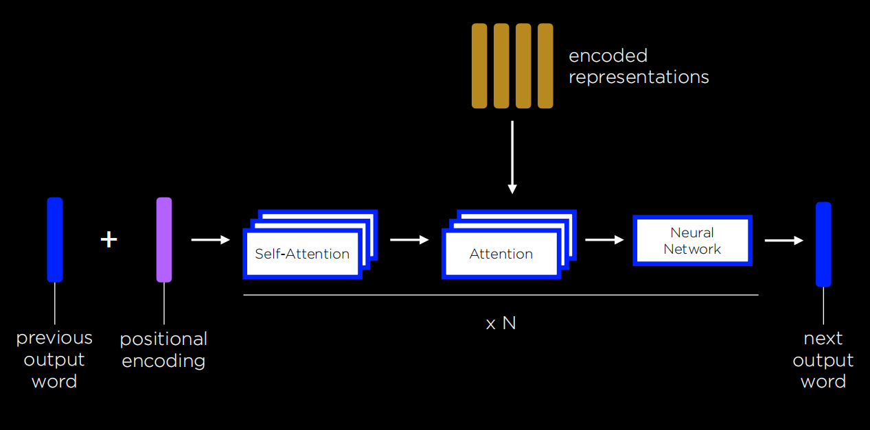
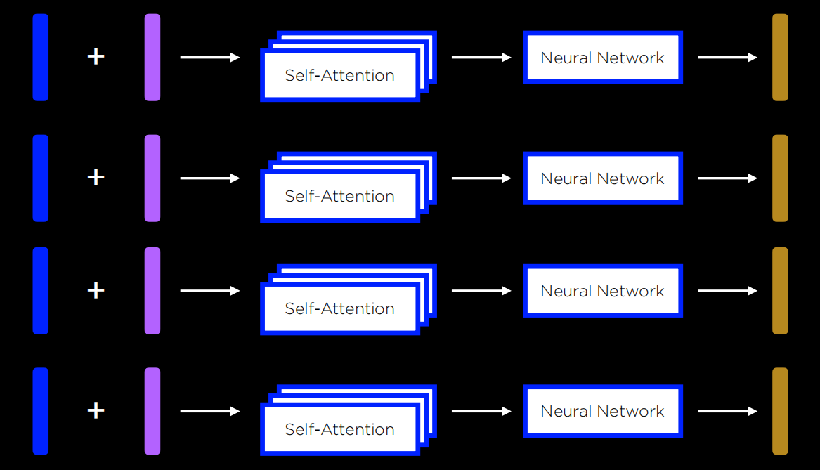
Transformers is a new type of training architecture whereby each input word is passed through a neural network simultaneously. An input word goes into the neural network and is captured as an encoded representation. Because all words are fed into the neural network at the same time, word order could easily be lost. Accordingly, position encoding is added to the inputs. The neural network, therefore, will use both the word and the position of the word in the encoded representation. Additionally, a self-attention step is added to help define the context of the word being inputted.

Encode:

Decode: